Effect Estimation with Intervention#
This example uses the Lalonde job training dataset, a classic benchmark for causal
inference with observational confounding, to estimate the effect of a job training
program on earnings.
The model encodes treatment as a NumPyro sample() site and
uses the intervention keyword to apply NumPyro’s
do handler, fixing treatment to specific values and
generating counterfactual predictions without rewriting the model.
The model includes a treatment x covariate interaction, decomposing the overall average treatment effect (ATE) into subgroup-specific conditional average treatment effects (CATEs) to ask whether the program helped those without a high-school degree more than those with one.
import logging

import arviz_base as az
import arviz_plots as azp
import arviz_stats as azs
import jax
import jax.numpy as jnp
import matplotlib.pyplot as plt
import numpy as np
import numpyro.distributions as dist
import pandas as pd
from jax import Array, random
from numpyro import deterministic, plate, sample
from numpyro.infer import MCMC, NUTS

from aimz import ImpactModel

logging.basicConfig(level=logging.INFO, force=True)

# Force JAX to use CPU even if GPU is available
jax.config.update("jax_platform_name", "cpu")
# Set the number of CPU devices JAX sees (for CPU-based parallelism)
jax.config.update("jax_num_cpu_devices", 2)

# Configure the inline backend for high-resolution figures
%config InlineBackend.figure_format = "retina"

# Set the style for ArviZ plots
azp.style.use("arviz-variat")

# Set a random seed for reproducibility
rng_key = random.key(532)
The Lalonde Dataset#
The dataset comes from an observational study of a job training program.
A total of 614 individuals were observed, of whom 185 received training and 429 did not.
The outcome is earnings in 1978 (re78), measured in thousands of dollars.
url = (
    "https://raw.githubusercontent.com/robjellis/lalonde/"
    "master/lalonde_data.csv"
)
df = pd.read_csv(url)

# Scale earnings to $k
df["re75"] = df["re75"] / 1_000
df["re78"] = df["re78"] / 1_000
The dataset contains the following columns:
Covariates (pre-treatment):
educ: years of education.age: age in years.re75: earnings in 1975, in thousands of dollars.black,hispan: race/ethnicity indicators.married: marital status indicator.nodegree: 1 if no high-school degree, 0 otherwise.
Treatment:
treat, 1 if the individual received job training.Outcome:
re78, earnings in 1978 (dollars, scaled to $k above).
The naive difference in mean earnings between the treated and control groups:
covariates = [
    "educ",
    "age",
    "re75",
    "black",
    "hispan",
    "married",
    "nodegree",
]
naive_ate = (
    df.loc[df["treat"] == 1, "re78"].mean() - df.loc[df["treat"] == 0, "re78"].mean()
)
print(f"Naive ATE: ${naive_ate:.3f}k")
Naive ATE: $-0.635k
The naive estimate is negative, suggesting the program reduced earnings. This is due to confounding: the treated group had lower prior earnings, less education, and other systematic differences.
df.groupby("treat")[covariates].mean().round(2).T
| treat | 0 | 1 |
|---|---|---|
| educ | 10.24 | 10.35 |
| age | 28.03 | 25.82 |
| re75 | 2.47 | 1.53 |
| black | 0.20 | 0.84 |
| hispan | 0.14 | 0.06 |
| married | 0.51 | 0.19 |
| nodegree | 0.60 | 0.71 |
fig, axes = plt.subplots(1, 2, figsize=(12, 4))

for treat_val, color, label in [(0, "C0", "Control"), (1, "C1", "Treated")]:
    subset = df.loc[df["treat"] == treat_val, "re78"]
    axes[0].hist(
        subset,
        alpha=0.5,
        color=color,
        label=label,
        density=True,
    )
axes[0].set(xlabel="Earnings 1978 ($k)", ylabel="Density")
axes[0].legend()

# Breakdown by nodegree x treatment
for (nd, treat), grp in df.groupby(["nodegree", "treat"]):
    label = f"{'No Degree' if nd else 'Degree'}, {'Treated' if treat else 'Control'}"
    axes[1].hist(grp["re78"], alpha=0.5, label=label, density=True)
axes[1].set(xlabel="Earnings 1978 ($k)", ylabel="Density")
axes[1].legend();
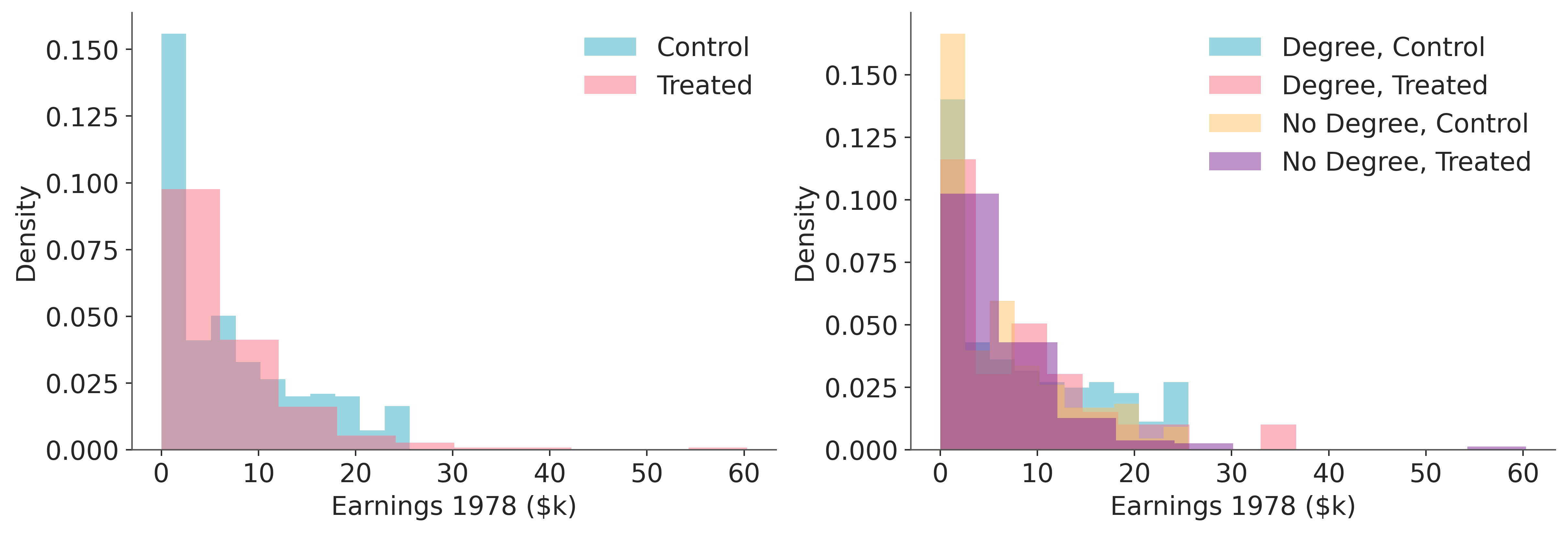
The right panel hints at heterogeneity: the earnings distributions differ more across treatment status for those without a degree than for those with one.
# Standardize continuous covariates for better sampling
cols_to_standardize = ["educ", "age", "re75"]
df[cols_to_standardize] = (
    df[cols_to_standardize] - df[cols_to_standardize].mean()
) / df[cols_to_standardize].std(ddof=0)

# Build JAX arrays
X = jnp.asarray(df[covariates].to_numpy(), dtype=jnp.float32)
y_treat = jnp.asarray(df["treat"].to_numpy(), dtype=jnp.int32)
y_earnings = jnp.asarray(df["re78"].to_numpy(), dtype=jnp.float32)
Model: Heterogeneous Treatment Effects#
The model includes a treatment x nodegree interaction, which allows the treatment
effect to differ between those without a high-school degree (nodegree = 1) and those
with one (nodegree = 0).
We employ a normal likelihood for simplicity, which keeps the treatment effect directly
interpretable in dollars.
The treatment variable treat is a sample() site, observed
during fitting (obs=y_treat) and intervened on during counterfactual prediction via
intervention.
n_obs, n_features = X.shape
nodegree_idx = covariates.index("nodegree")


def earnings_model(
    X: Array,
    y: Array | None = None,
    y_treat: Array | None = None,
) -> None:
    # Treatment sub-model: makes treat a sample site so that the
    # intervention keyword can fix its value via do().
    p_treat = sample("p_treat", dist.Beta(1.0, 1.0))
    with plate("obs_treat", n_obs):
        treat = sample("treat", dist.Bernoulli(probs=p_treat), obs=y_treat)

    # Outcome model with heterogeneous treatment effect.
    # Priors are weakly informative relative to the data scale.
    intercept = sample("intercept", dist.Normal(0.0, 5.0))
    beta_treat = sample("beta_treat", dist.Normal(0.0, 2.0))
    beta_interact = sample("beta_interact", dist.Normal(0.0, 2.0))
    beta_cov = sample(
        "beta_cov",
        dist.Normal(0.0, 1.0).expand([n_features]),
    )
    sigma = sample("sigma", dist.HalfNormal(5.0))

    nodegree = X[:, nodegree_idx]
    mu = intercept + (beta_treat + beta_interact * nodegree) * treat + X @ beta_cov
    deterministic("mu_earnings", mu)

    with plate("obs", n_obs):
        sample("y", dist.Normal(mu, sigma), obs=y)
The linear predictor expands to
intercept + beta_treat * treat + beta_interact * treat * nodegree + X @ beta_cov.
The treatment effect for a degree holder (nodegree = 0) is beta_treat, and for
a non-degree holder (nodegree = 1) it is beta_treat + beta_interact.
The treatment sub-model is intentionally simple: it does not model the treatment
assignment mechanism.
Its purpose is to make treat a sample site so that intervention can fix
treatment values via NumPyro’s do handler.
Causal identification relies on the outcome regression: under conditional ignorability
and correct specification of the outcome model, the average over individual-level
counterfactual predictions recovers the ATE.
This is sometimes called g-computation.
If the outcome model is misspecified, the resulting ATE may be biased; in practice,
flexible outcome models or doubly robust estimators can reduce this risk.
We fit using MCMC with the No-U-Turn Sampler.
rng_key, rng_subkey = random.split(rng_key)
im = ImpactModel(
    earnings_model,
    rng_key=rng_subkey,
    inference=MCMC(
        NUTS(earnings_model),
        num_warmup=500,
        num_samples=500,
        num_chains=2,
    ),
)

im.fit_on_batch(X, y_earnings, y_treat=y_treat)
MCMC diagnostics:
summary = azs.summary(az.from_numpyro(im.inference))
summary.loc[~summary.index.str.startswith("mu_earnings")]
| mean | sd | eti89_lb | eti89_ub | ess_bulk | ess_tail | r_hat | mcse_mean | mcse_sd | |
|---|---|---|---|---|---|---|---|---|---|
| beta_cov[0] | 1.17 | 0.35 | 0.62 | 1.7 | 805 | 747 | 1.00 | 0.012 | 0.0087 |
| beta_cov[1] | 0.52 | 0.29 | 0.049 | 0.97 | 1496 | 849 | 1.00 | 0.0075 | 0.0052 |
| beta_cov[2] | 1.53 | 0.28 | 1.1 | 2 | 1429 | 758 | 1.01 | 0.0075 | 0.0052 |
| beta_cov[3] | -0.97 | 0.6 | -1.9 | 0.0085 | 1418 | 924 | 1.00 | 0.016 | 0.011 |
| beta_cov[4] | 0.25 | 0.69 | -0.85 | 1.3 | 1798 | 852 | 1.01 | 0.016 | 0.012 |
| beta_cov[5] | 0.84 | 0.56 | -0.056 | 1.8 | 1086 | 762 | 1.01 | 0.017 | 0.012 |
| beta_cov[6] | 0.09 | 0.68 | -0.97 | 1.2 | 713 | 754 | 1.00 | 0.026 | 0.016 |
| beta_interact | -0.72 | 1.04 | -2.4 | 0.95 | 861 | 728 | 1.01 | 0.035 | 0.025 |
| beta_treat | 1.21 | 0.95 | -0.32 | 2.7 | 836 | 774 | 1.01 | 0.033 | 0.024 |
| intercept | 6.51 | 0.65 | 5.5 | 7.5 | 650 | 720 | 1.00 | 0.025 | 0.017 |
| p_treat | 0.3026 | 0.0189 | 0.27 | 0.33 | 2083 | 814 | 1.00 | 0.00042 | 0.00033 |
| sigma | 7.083 | 0.202 | 6.8 | 7.4 | 1824 | 691 | 1.01 | 0.0048 | 0.0033 |
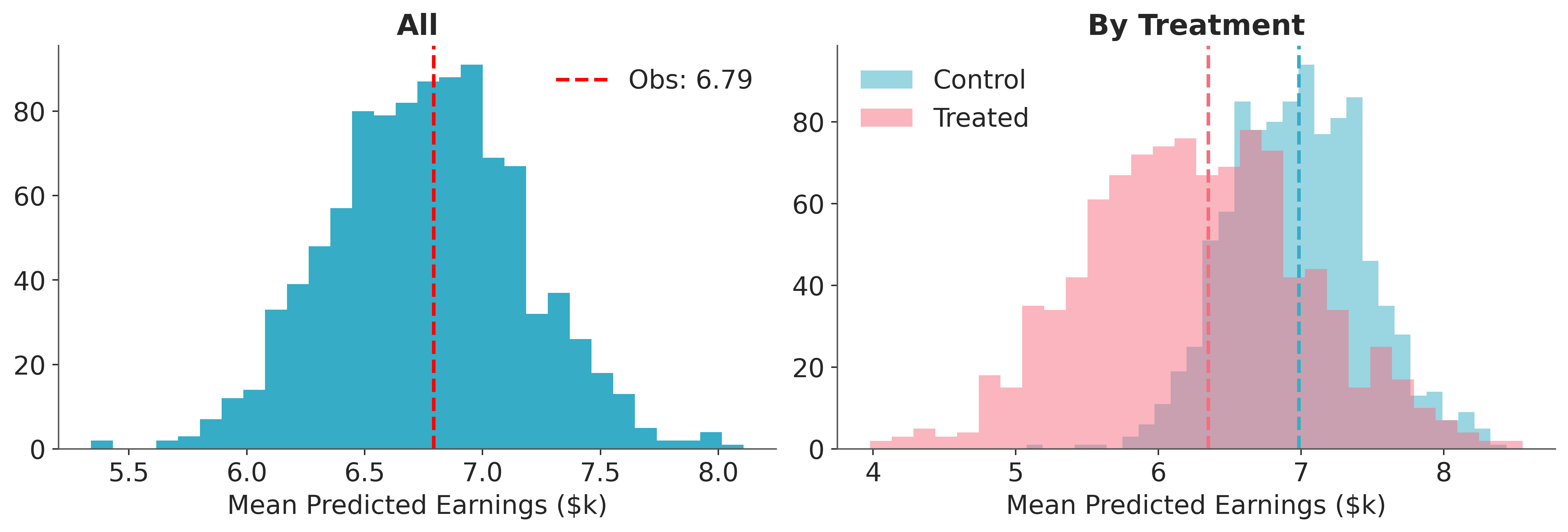
Posterior Predictive Check#
The posterior predictive check below compares the observed and predicted mean earnings overall and by treatment arm.
dt = im.predict_on_batch(X, y_treat=y_treat)
pp_earn = dt.posterior_predictive["y"]

fig, axes = plt.subplots(1, 2, figsize=(12, 4))

# Overall
obs_mean = float(y_earnings.mean())
pred_means = pp_earn.mean(dim="y_dim_0").to_numpy().flatten()
axes[0].hist(pred_means, bins=30, color="C0")
axes[0].axvline(
    obs_mean,
    color="red",
    linestyle="--",
    linewidth=2,
    label=f"Obs: {obs_mean:.2f}",
)
axes[0].set(xlabel="Mean Predicted Earnings ($k)", title="All")
axes[0].legend()

# Per treatment arm
for arm, color in [(0, "C0"), (1, "C1")]:
    mask = np.asarray(y_treat == arm)
    obs_arm = float(y_earnings[mask].mean())
    pred_arm = pp_earn.isel(y_dim_0=mask).mean(dim="y_dim_0").to_numpy().flatten()
    axes[1].hist(
        pred_arm,
        bins=30,
        color=color,
        alpha=0.5,
        label=f"{'Treated' if arm else 'Control'}",
    )
    axes[1].axvline(obs_arm, color=color, linestyle="--", linewidth=2)
axes[1].set(xlabel="Mean Predicted Earnings ($k)", title="By Treatment")
axes[1].legend();
Estimating Treatment Effects via intervention#
Because treat is a sample() site rather than a regular
function argument, we use the intervention keyword inside the scenario dicts.
This triggers NumPyro’s do handler, which severs
the incoming edges to the treat node, generating counterfactual predictions under
fixed treatment values.
effect = im.estimate_effect(
    args_baseline={
        "X": X,
        "intervention": {"treat": jnp.zeros(n_obs, dtype=jnp.int32)},
    },
    args_intervention={
        "X": X,
        "intervention": {"treat": jnp.ones(n_obs, dtype=jnp.int32)},
    },
    on_batch=True,
)
The result contains individual-level differences (intervention − baseline) for
mu_earnings.
Averaging over all observations gives the overall ATE.
ite = effect.posterior_predictive["mu_earnings"]
ate = ite.mean(dim="mu_earnings_dim_0")
Overall ATE#
fig, ax = plt.subplots(figsize=(8, 4))

pp_ate = ate.to_numpy().flatten()
ax.hist(pp_ate, bins=30, color="C0")
ax.axvline(
    pp_ate.mean(),
    color="red",
    linestyle="--",
    linewidth=2,
    label=f"Mean: {pp_ate.mean():.2f}",
)
ax.axvline(0, color="gray", linestyle=":")
ax.set(xlabel="ATE ($k)", ylabel="Frequency")
ax.legend()
fig.suptitle("Overall Average Treatment Effect", fontweight="bold");
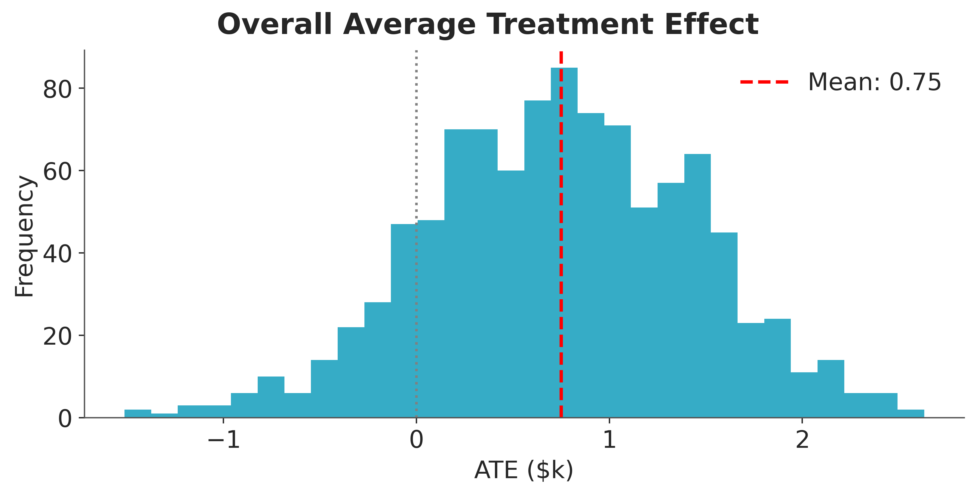
The posterior mean is positive, indicating that the training program increased earnings on average. The interval is wide and includes zero, reflecting the small sample size, high variance of individual earnings, and imbalanced treatment groups.
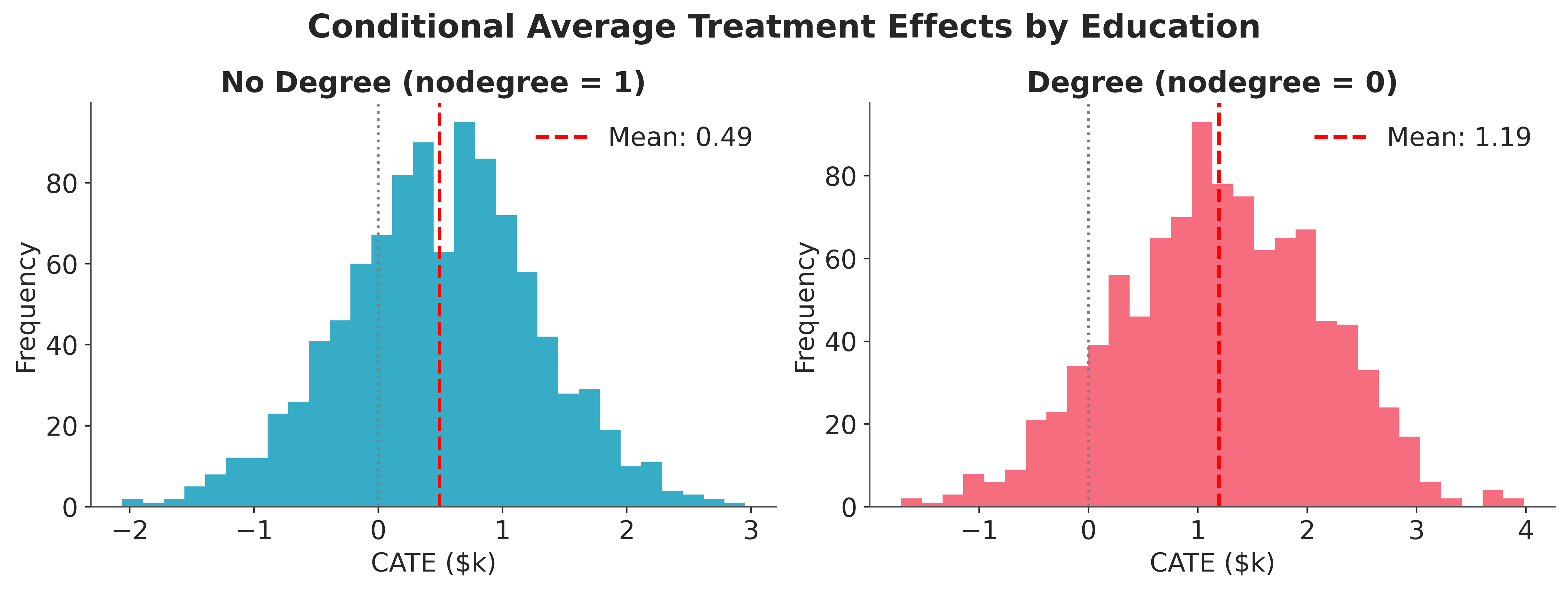
Subgroup CATEs#
Because the model includes a treatment x nodegree interaction, the individual-level
treatment effects vary by subgroup.
We partition the observations and average each subset.
nodegree_mask = np.asarray(df["nodegree"] == 1)

cate_no_degree = ite.isel(mu_earnings_dim_0=nodegree_mask).mean(dim="mu_earnings_dim_0")
cate_degree = ite.isel(mu_earnings_dim_0=~nodegree_mask).mean(dim="mu_earnings_dim_0")
fig, axes = plt.subplots(1, 2, figsize=(12, 4), layout="constrained")

for i, (ax, draws, label) in enumerate(zip(
    axes,
    [cate_no_degree, cate_degree],
    ["No Degree (nodegree = 1)", "Degree (nodegree = 0)"],
    strict=True,
)):
    pp = draws.to_numpy().flatten()
    ax.hist(pp, bins=30, color=f"C{i}")
    mean = pp.mean()
    ax.axvline(
        mean, color="red", linestyle="--", linewidth=2,
        label=f"Mean: {mean:.2f}",
    )
    ax.axvline(0, color="gray", linestyle=":")
    ax.set_title(label)
    ax.set_xlabel("CATE ($k)")
    ax.set_ylabel("Frequency")
    ax.legend()

fig.suptitle(
    "Conditional Average Treatment Effects by Education",
    fontsize=18,
    fontweight="bold",
    y=1.1,
);
fig, ax = plt.subplots(figsize=(8, 4))

labels = []
for i, (draws, label) in enumerate(
    zip(
        [ate, cate_no_degree, cate_degree],
        ["Overall ATE", "CATE: No Degree", "CATE: Degree"],
        strict=True,
    ),
):
    pp = draws.to_numpy().flatten()
    mean = pp.mean()
    hdi = azs.hdi(pp)
    ax.errorbar(
        mean,
        i,
        xerr=[[mean - hdi[0]], [hdi[1] - mean]],
        fmt="o",
        capsize=5,
        color=f"C{i}",
        markersize=8,
    )
    labels.append(label)
ax.set_yticks(range(len(labels)))
ax.set_yticklabels(labels)
ax.axvline(0, color="gray", linestyle=":")
ax.set_xlabel("Treatment Effect ($k)")
ax.set_title("Treatment Effect Comparison", fontweight="bold");
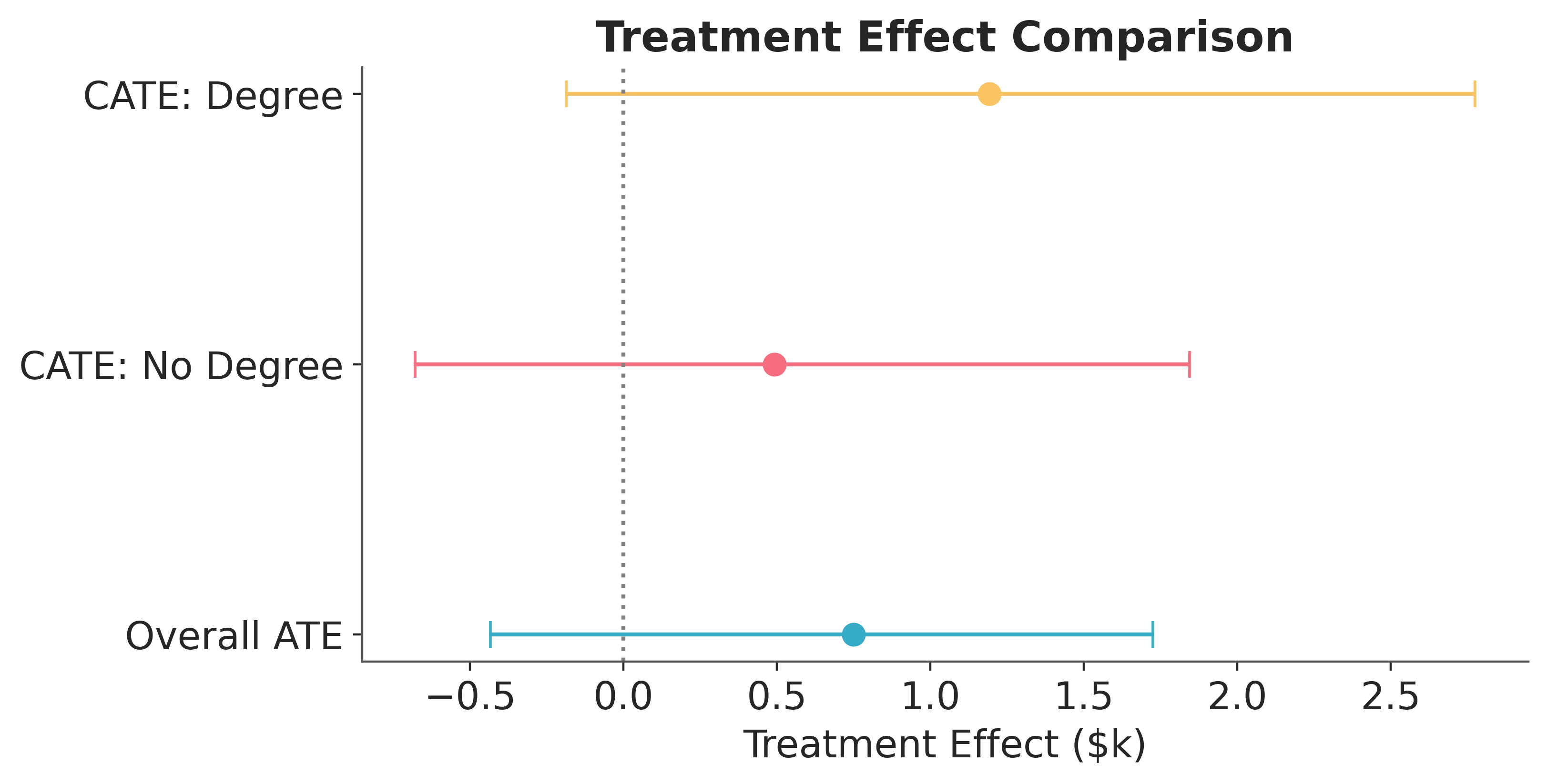
The plot compares the overall ATE with subgroup CATEs.
This decomposition is a direct consequence of the interaction term; the same
estimate_effect call produces both through post-processing.
For this linear model, the subgroup CATEs could also be read directly from the
coefficients, but the workflow shown here generalizes to models where the treatment
effect has no closed-form expression.
All three intervals include zero, so the data do not provide strong evidence that the program increased earnings for either subgroup. The degree-holder CATE has a larger point estimate than the no-degree CATE, but its interval is also wider, in part because there are fewer degree holders in the treated group. The two CATEs overlap substantially, meaning the data do not support a confident claim of treatment effect heterogeneity by education level.
The subgroup CATEs are determined by the interaction structure in the model, not discovered from the data nonparametrically. A richer model with additional interactions or flexible components could reveal different patterns of heterogeneity.
References#
Dehejia, R. and Wahba, S. (1999). Causal Effects in Non-Experimental Studies: Reevaluating the Evaluation of Training Programs. Journal of the American Statistical Association, 94(448), 1053–1062.
Dehejia, R. and Wahba, S. (2002). Propensity Score Matching Methods for Non-Experimental Causal Studies. Review of Economics and Statistics, 84(1), 151–161.
Lalonde, R. (1986). Evaluating the Econometric Evaluations of Training Programs. American Economic Review, 76(4), 604–620.