Scalable Predictive Sampling#
This example uses the Criteo Uplift Prediction dataset,
a large-scale advertising benchmark with approximately 14 million observations, to
demonstrate aimz’s scalable inference pipeline: minibatch stochastic variational
inference (SVI) with fit(), streaming posterior predictive
sampling to Zarr with predict(), and deterministic resource
cleanup with cleanup().
The model is a Bayesian neural network (BNN) built with
Flax and lifted into NumPyro through
random_nnx_module().
Treatment is passed as an input feature, and the ImpactModel API handles
batched training and prediction without requiring changes to the model code.
import logging

import jax
import jax.numpy as jnp
import matplotlib.pyplot as plt
import numpy as np
import numpyro.distributions as dist
import pandas as pd
from flax import nnx
from jax import Array, default_backend, random
from jax.typing import ArrayLike
from numpyro import deterministic, plate, sample
from numpyro.contrib.module import random_nnx_module
from numpyro.infer import SVI, Trace_ELBO, init_to_uniform
from numpyro.infer.autoguide import AutoNormal
from optax import adam

from aimz import ImpactModel

logging.basicConfig(level=logging.INFO, force=True)

# Configure the inline backend for high-resolution figures
%config InlineBackend.figure_format = "retina"

# Set a random seed for reproducibility
rng_key = random.key(532)
The Criteo Uplift Dataset#
The Criteo Uplift Prediction dataset (v2.1) was constructed from several randomized
incrementality tests in online advertising.
In each test, a random subset of users was withheld from ad targeting (control) while
the remainder was eligible for ads (treated).
The treatment group is deliberately large (~85%) because withholding ads from control
users has a direct revenue cost.
The dataset contains approximately 14 million rows, each corresponding to a user with 12
anonymized features (f0 through f11), a binary treatment indicator, and two
binary outcomes.
The dataset is also available from
Hugging Face
(~300 MB compressed).
df = pd.read_parquet("criteo.parquet")
The dataset contains the following columns:
Features:
f0throughf11, 12 dense float-valued covariates. Feature names are anonymized and values are randomly projected to preserve predictive power while preventing recovery of the original user context.Treatment:
treatment, binary indicator (1 = user was eligible for ad targeting, 0 = withheld from targeting). Note thattreatment = 1does not guarantee the user saw an ad; it means they were eligible for targeting in the real-time bidding auction.Exposure:
exposure, binary indicator of whether the user was actually shown an ad. By construction,treatment = 0impliesexposure = 0. Because exposure occurs after treatment assignment and depends on auction dynamics, conditioning on it would introduce post-treatment bias. The analysis usestreatmentalone, yielding an intention-to-treat (ITT) estimate.Outcomes:
visit: whether the user visited the advertiser’s site (binary, ~4.7%).conversion: whether a purchase occurred (binary, ~0.3%). By construction,visit = 0impliesconversion = 0.
We model visit as the outcome because its higher base rate (~4.7% vs.
~0.3%) makes the treatment effect easier to detect. The conversion outcome
could be modeled with the same workflow.
print(f"Rows: {len(df):,}")
print(f"Visit rate: {df['visit'].mean():.4f}")
print(f"Conversion rate: {df['conversion'].mean():.5f}")
print(f"Treatment ratio: {df['treatment'].mean():.2f}")
Rows: 13,979,592
Visit rate: 0.0470
Conversion rate: 0.00292
Treatment ratio: 0.85
feature_cols = [f"f{i}" for i in range(12)]
n_obs = len(df)

X = jnp.asarray(df[feature_cols].to_numpy(), dtype=jnp.float32)
treatment = jnp.asarray(df["treatment"].to_numpy(), dtype=jnp.float32)
y_visit = jnp.asarray(df["visit"].to_numpy(), dtype=jnp.int32)
Model: Bayesian Neural Network#
The model is a three-layer multilayer perceptron (MLP) with ReLU activations. The architecture is intentionally small (32 hidden units) to keep training fast. Treatment is concatenated with the 12 features as an input column, making this an S-learner: a single model that learns the conditional outcome distribution as a function of both covariates and treatment status.
random_nnx_module() places a prior over the
network parameters, and the plate construct with subsample_size enables
minibatch SVI by scaling the log-likelihood contribution of each batch to the full
dataset.
class MLP(nnx.Module):
    dtype: jnp.dtype = jnp.bfloat16 if default_backend() == "gpu" else jnp.float32

    def __init__(self, din: int, dmid: int, dout: int, *, rngs: nnx.Rngs) -> None:
        self.linear1 = nnx.Linear(din, dmid, dtype=self.dtype, rngs=rngs)
        self.linear2 = nnx.Linear(dmid, dmid, dtype=self.dtype, rngs=rngs)
        self.linear3 = nnx.Linear(dmid, dout, dtype=self.dtype, rngs=rngs)

    def __call__(self, x: ArrayLike) -> Array:
        x = nnx.relu(self.linear1(x))
        x = nnx.relu(self.linear2(x))

        return self.linear3(x).squeeze()


rng_key, rng_subkey = random.split(rng_key)
nn_module = MLP(
    din=13,  # 12 features + 1 treatment indicator
    dmid=32,
    dout=1,
    rngs=nnx.Rngs(params=rng_subkey),
)


def visit_model(
    X: ArrayLike,
    treatment: ArrayLike,
    *,
    y: ArrayLike | None = None,
) -> None:
    nn_p = random_nnx_module(
        "nn_p",
        nn_module=nn_module,
        scope_divider="_",
        prior=dist.Normal(),
    )
    X_aug = jnp.column_stack([X, treatment[:, None]])
    with plate("data", size=n_obs, subsample_size=len(X)):
        logits = nn_p(X_aug)
        deterministic("p", nnx.sigmoid(logits))
        sample("y", dist.Bernoulli(logits=logits), obs=y)
The network outputs logits, which are passed to Bernoulli(logits=...).
The 13th input column is the treatment indicator.
During counterfactual prediction, changing this column from 0 to 1 (or vice versa)
produces predictions under the alternative treatment scenario.
The plate("data", size=n_obs, subsample_size=len(X)) construct declares that the
current batch is a subsample of n_obs total observations.
During minibatch training, fit() passes minibatches to the
model, so len(X) equals the current batch size and the plate scales each batch’s
log-likelihood to the full dataset.
During prediction, the full array is passed and len(X) equals n_obs.
Training#
The fit() method performs minibatch SVI updates.
Unlike fit_on_batch(), it processes data in batches of
batch_size over multiple epochs, updating the variational parameters according
to the configured optimization strategy.
After optimization, it draws num_samples posterior samples from the fitted guide.
We use 100 samples here for illustration; more samples would tighten the posterior
estimates.
rng_key, rng_subkey = random.split(rng_key)
im = ImpactModel(
    visit_model,
    rng_key=rng_subkey,
    inference=SVI(
        visit_model,
        guide=AutoNormal(
            model=visit_model,
            init_loc_fn=init_to_uniform(radius=0.1),
        ),
        optim=adam(learning_rate=1e-3),
        loss=Trace_ELBO(),
    ),
)
im.fit(
    X,
    treatment=treatment,
    y=y_visit,
    num_samples=100,
    batch_size=4096,
    epochs=10,
);
Performing variational inference optimization...
Epoch 1/10 - Average loss: 2310007.0000
Epoch 2/10 - Average loss: 1790094.3750
Epoch 3/10 - Average loss: 1716746.8750
Epoch 4/10 - Average loss: 1672026.3750
Epoch 5/10 - Average loss: 1647541.8750
Epoch 6/10 - Average loss: 1631482.8750
Epoch 7/10 - Average loss: 1617123.1250
Epoch 8/10 - Average loss: 1603617.7500
Epoch 9/10 - Average loss: 1590345.8750
Epoch 10/10 - Average loss: 1579658.5000
Posterior sampling...
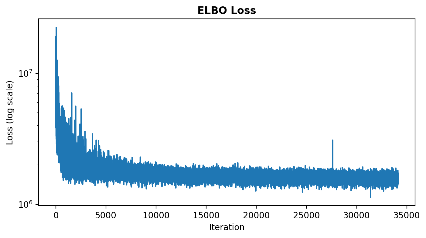
The ELBO loss history is stored in im.vi_result.losses.
fig, ax = plt.subplots(figsize=(8, 4))
ax.plot(im.vi_result.losses)
ax.set(yscale="log", xlabel="Iteration", ylabel="Loss (log scale)")
ax.set_title("ELBO Loss", fontweight="bold")
Streaming Prediction#
The predict() method streams posterior predictive samples to
Zarr, a chunked array format that supports out-of-core access.
With 100 posterior samples and 14 million observations, the posterior predictive array
contains over 1.4 billion values.
Rather than materializing this array in memory, predict() writes
results incrementally in chunks of batch_size, keeping memory usage constant
regardless of dataset size and bounding host-to-device transfers on accelerators.
Computation is JIT-compiled and automatically sharded across available devices.
dt = im.predict(X, treatment=treatment)
The return value is an xarray.DataTree backed by Zarr stores on disk.
Downstream analysis can slice and aggregate without loading the full array into memory.
We verify the model fit by comparing the observed visit rate against the posterior predictive distribution, both overall and per treatment arm.
pp_visit = dt.posterior_predictive["y"]

fig, axes = plt.subplots(1, 3, figsize=(12, 4))

# Overall
obs_rate = float(y_visit.mean())
pred_rate = pp_visit.mean(dim="y_dim_0").to_numpy().flatten()
axes[0].hist(pred_rate, bins=20, color="C0")
axes[0].axvline(
    obs_rate,
    color="red",
    linestyle="--",
    linewidth=2,
    label=f"Obs: {obs_rate:.4f}",
)
axes[0].set(xlabel="Mean Predicted Visit Rate", ylabel="Frequency", title="All")
axes[0].legend()

# Per treatment arm
for i, (arm_val, label) in enumerate([(0, "Control"), (1, "Treated")]):
    mask = np.asarray(treatment == arm_val)
    obs_arm = float(np.asarray(y_visit)[mask].mean())
    pred_arm = pp_visit.isel(y_dim_0=mask).mean(dim="y_dim_0").to_numpy().flatten()
    axes[i + 1].hist(pred_arm, bins=20, color=f"C{i + 1}")
    axes[i + 1].axvline(
        obs_arm,
        color="red",
        linestyle="--",
        linewidth=2,
        label=f"Obs: {obs_arm:.4f}",
    )
    axes[i + 1].set(xlabel="Mean Predicted Visit Rate", title=label)
    axes[i + 1].legend()

fig.suptitle("Posterior Predictive Check: Visit Rate", fontweight="bold", y=1.05);
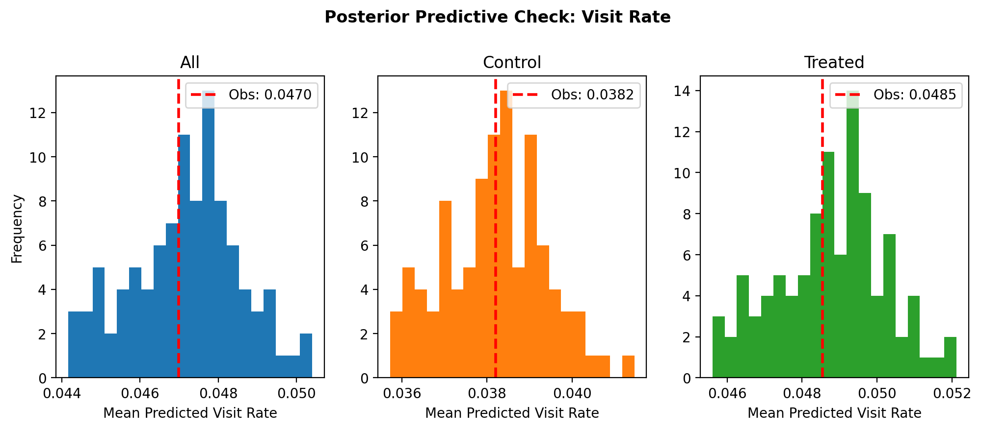
The observed visit rate falls within the posterior predictive distribution in all three panels, and the model captures the gap between the control and treated groups.
Treatment Effect Estimation#
Because the dataset comes from a randomized experiment, the average treatment effect on
visit probability can be estimated by predicting under both treatment scenarios and
averaging the difference.
The treatment column indicates eligibility for ad targeting rather than guaranteed
ad exposure, so the estimated effect is an intention-to-treat (ITT) effect: the impact
of allowing users to enter the ad auction, not the causal effect of actually viewing an
ad.
Treatment is a function argument (not a sample site), so
estimate_effect() runs predict() twice
with different treatment values.
Alternatively, precomputed prediction outputs can be passed directly to avoid
computation internally.
effect = im.estimate_effect(
    args_baseline={
        "X": X,
        "treatment": jnp.zeros(n_obs, dtype=jnp.float32),
    },
    args_intervention={
        "X": X,
        "treatment": jnp.ones(n_obs, dtype=jnp.float32),
    },
)

ate = effect.posterior_predictive["p"].mean(dim="p_dim_0")
fig, ax = plt.subplots(figsize=(8, 4))
pp_ate = ate.to_numpy().flatten()
ax.hist(pp_ate, bins=20)
ax.axvline(
    pp_ate.mean(),
    color="red",
    linestyle="--",
    linewidth=2,
    label=f"Mean: {pp_ate.mean():.4f}",
)
ax.set(xlabel="ATE (Visit Probability)", ylabel="Frequency")
ax.legend()
ax.set_title("Average Treatment Effect on Visit", fontweight="bold");
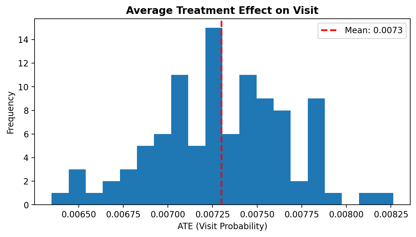
The difference-in-means provides a simple benchmark for comparison:
naive_ate = (
    df.loc[df["treatment"] == 1, "visit"].mean()
    - df.loc[df["treatment"] == 0, "visit"].mean()
)
print(f"Difference-in-means: {naive_ate:.4f}")
print(f"Model:               {pp_ate.mean():.4f}")
Difference-in-means: 0.0103
Model:               0.0073
Cleanup#
When predict() writes to a temporary directory (the default when
no output_dir is specified), cleanup() releases the disk
resources.
This is optional but recommended in long-running sessions.
im.cleanup()
References#
Diemert, E., Betlei, A., Renaudin, C., and Amini, M.-R. (2018). A Large Scale Benchmark for Uplift Modeling. Proceedings of the AdKDD and TargetAd Workshop, KDD 2018.