Explicit Sampling#
aimz provides three sets of explicit sampling methods from the ImpactModel class, similar to PyMC samplers:
Prior Predictive Sampling:
sample_prior_predictive_on_batch()andsample_prior_predictive().Posterior Sampling:
sample().Posterior Predictive Sampling:
sample_posterior_predictive_on_batch()andsample_posterior_predictive().
By default, these methods return results as an xarray.DataTree, with the relevant group labeled as prior_predictive, posterior, or posterior_predictive.
For some methods, setting return_datatree=False instead returns a dict.
The prior predictive sampling methods perform forward sampling based on the model’s prior specification in the kernel and are not part of the standard training and inference workflow (fit()/predict()), making them particularly useful for conducting prior predictive checks.
Unlike fit() or fit_on_batch(), sample() does not modify the internal posterior attribute.
It is primarily intended for drawing posterior samples from a fitted model using variational inference.
Users can update the internal posterior manually by passing the samples obtained from sample() to set_posterior_sample() without retraining the model.
The posterior predictive sampling methods serve as convenient aliases for predict_on_batch() and predict(), respectively.
import logging

import jax.numpy as jnp
import numpyro.distributions as dist
import xarray as xr
from arviz_plots import plot_ppc_dist, style
from jax import random
from jax.typing import ArrayLike
from numpyro import optim, plate, sample
from numpyro.infer import SVI, Trace_ELBO
from numpyro.infer.autoguide import AutoNormal

from aimz import ImpactModel

logging.basicConfig(level=logging.INFO, force=True)
style.use("arviz-variat")
A minimal linear regression model and synthetic data are defined as an example below.
def model(X: ArrayLike, y: ArrayLike | None = None) -> None:
    """Linear regression model."""
    w = sample("w", dist.Normal().expand((X.shape[1],)))
    b = sample("b", dist.Normal())
    mu = jnp.dot(X, w) + b
    sigma = sample("sigma", dist.Exponential())
    with plate("data", size=X.shape[0]):
        sample("y", dist.Normal(mu, sigma), obs=y)


rng_key = random.key(42)
rng_key, rng_key_w, rng_key_b, rng_key_x, rng_key_e = random.split(rng_key, 5)
w = random.normal(rng_key_w, (5,))
b = random.normal(rng_key_b)
X = random.normal(rng_key_x, (1000, 5))
e = random.normal(rng_key_e, (1000,))
y = jnp.dot(X, w) + b + e


rng_key, rng_subkey = random.split(rng_key)
im = ImpactModel(
    model,
    rng_key=rng_subkey,
    inference=SVI(
        model,
        guide=AutoNormal(model),
        optim=optim.Adam(step_size=1e-3),
        loss=Trace_ELBO(),
    ),
)
Prior Predictive Sampling#
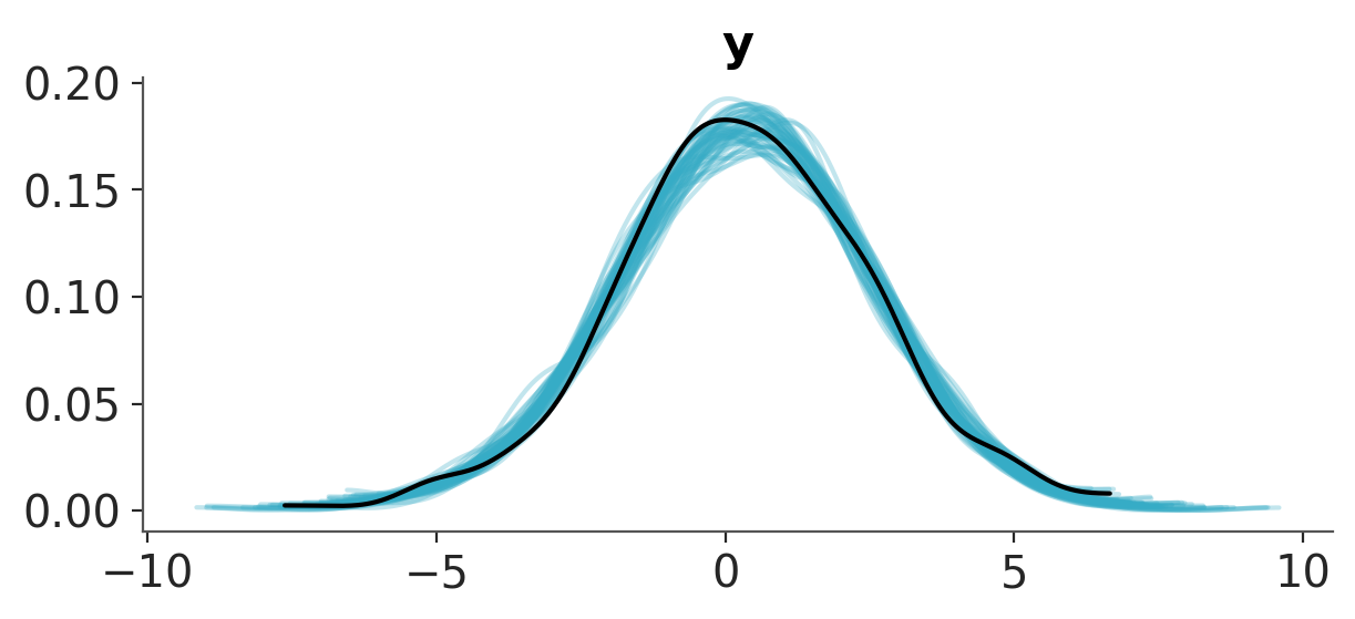
Before training the model, we draw prior predictive samples and visualize the prior predictive distribution:
dt = im.sample_prior_predictive_on_batch(X, num_samples=100)
plot_ppc_dist(dt, var_names="y", group="prior_predictive")
dt
<xarray.DataTree 'root'>
Group: /
└── Group: /prior_predictive
        Dimensions:  (chain: 1, draw: 100, y_dim_0: 1000)
        Coordinates:
          * chain    (chain) int64 8B 0
          * draw     (draw) int64 800B 0 1 2 3 4 5 6 7 8 ... 91 92 93 94 95 96 97 98 99
          * y_dim_0  (y_dim_0) int64 8kB 0 1 2 3 4 5 6 7 ... 993 994 995 996 997 998 999
        Data variables:
            y        (chain, draw, y_dim_0) float32 400kB -0.4827 0.5957 ... -0.3813
        Attributes:
            created_at:    2026-07-04T02:50:01.767917+00:00
            aimz_version:  0.13.0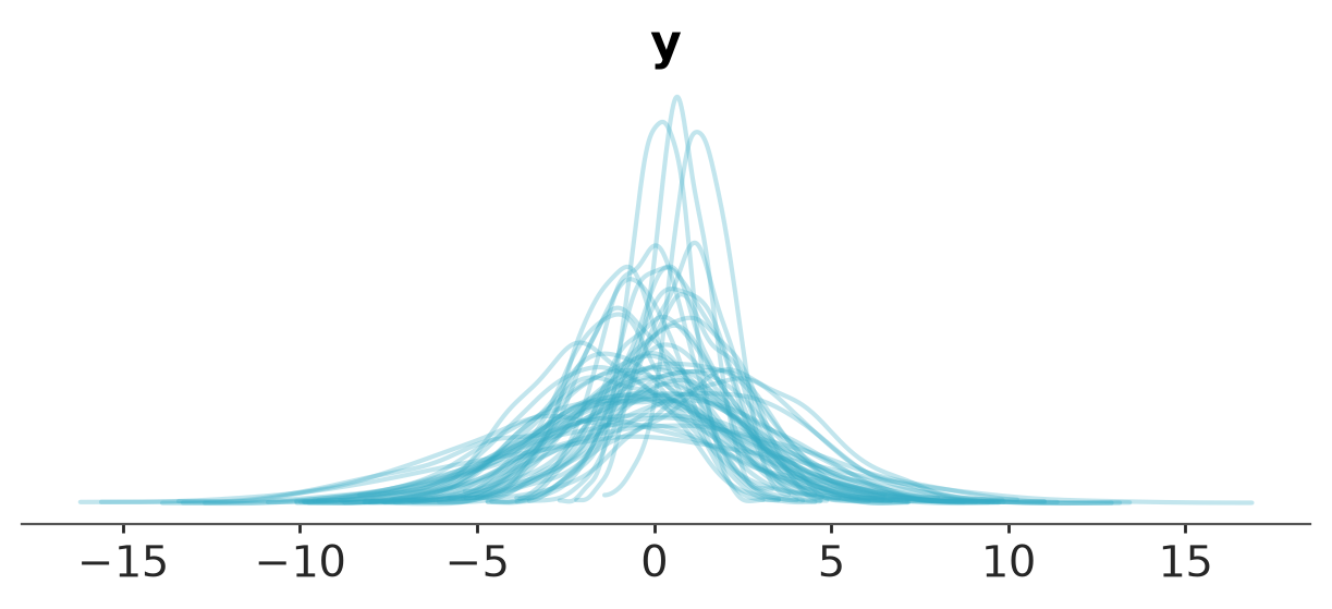
Posterior Sampling#
We first train the model using variational inference, drawing only a single posterior sample for demonstration purposes.
After fitting, we call sample() to generate 100 posterior samples for further analysis.
Setting return_datatree=False ensures that the results are returned as a dictionary rather than an xarray.DataTree.
im.fit_on_batch(X, y, num_samples=1, progress=False)
posterior_samples = im.sample(num_samples=100, return_datatree=False)
We pass posterior samples to set_posterior_sample() to update the model’s internal posterior:
im.set_posterior_sample(posterior_samples);
Posterior Predictive Sampling#
We draw posterior predictive samples from the fitted model using sample_posterior_predictive_on_batch(), though the same results can be obtained with predict_on_batch() (or predict()).
The posterior group now contains 100 posterior samples.
dt_posterior_predictive = im.sample_posterior_predictive_on_batch(X)
dt_posterior_predictive
<xarray.DataTree 'root'>
Group: /
├── Group: /posterior
│       Dimensions:  (chain: 1, draw: 100, w_dim_0: 5)
│       Coordinates:
│         * chain    (chain) int64 8B 0
│         * draw     (draw) int64 800B 0 1 2 3 4 5 6 7 8 ... 91 92 93 94 95 96 97 98 99
│         * w_dim_0  (w_dim_0) int64 40B 0 1 2 3 4
│       Data variables:
│           b        (chain, draw) float32 400B 0.3868 0.4323 0.4526 ... 0.485 0.3385
│           sigma    (chain, draw) float32 400B 1.043 1.067 1.053 ... 1.011 1.081 1.109
│           w        (chain, draw, w_dim_0) float32 2kB 0.5985 0.8279 ... -0.611 -1.199
│       Attributes:
│           created_at:    2026-07-04T02:50:07.174977+00:00
│           aimz_version:  0.13.0
└── Group: /posterior_predictive
        Dimensions:  (chain: 1, draw: 100, y_dim_0: 1000)
        Coordinates:
          * chain    (chain) int64 8B 0
          * draw     (draw) int64 800B 0 1 2 3 4 5 6 7 8 ... 91 92 93 94 95 96 97 98 99
          * y_dim_0  (y_dim_0) int64 8kB 0 1 2 3 4 5 6 7 ... 993 994 995 996 997 998 999
        Data variables:
            y        (chain, draw, y_dim_0) float32 400kB 0.1231 2.521 ... -0.2459 4.068
        Attributes:
            created_at:    2026-07-04T02:50:07.177301+00:00
aimz_version: 0.13.0We join the posterior_predictive group from dt_posterior_predictive to the dt containing the prior_predictive group, and also add the observed_data as a new group to visualize the posterior predictive distribution.
# Add posterior predictive samples as a new group
dt["/posterior_predictive"] = dt_posterior_predictive.posterior_predictive

# Create a dataset for observed data and add as a new group
ds = xr.Dataset({"y": xr.DataArray(y, dims=["y_dim_0"])})
dt["/observed_data"] = xr.DataTree(ds)

# Plot the posterior predictive distribution
plot_ppc_dist(dt, var_names="y")

# Display the combined DataTree
dt
<xarray.DataTree 'root'>
Group: /
├── Group: /prior_predictive
│       Dimensions:  (chain: 1, draw: 100, y_dim_0: 1000)
│       Coordinates:
│         * chain    (chain) int64 8B 0
│         * draw     (draw) int64 800B 0 1 2 3 4 5 6 7 8 ... 91 92 93 94 95 96 97 98 99
│         * y_dim_0  (y_dim_0) int64 8kB 0 1 2 3 4 5 6 7 ... 993 994 995 996 997 998 999
│       Data variables:
│           y        (chain, draw, y_dim_0) float32 400kB -0.4827 0.5957 ... -0.3813
│       Attributes:
│           created_at:    2026-07-04T02:50:01.767917+00:00
│           aimz_version:  0.13.0
├── Group: /posterior_predictive
│       Dimensions:  (chain: 1, draw: 100, y_dim_0: 1000)
│       Coordinates:
│         * chain    (chain) int64 8B 0
│         * draw     (draw) int64 800B 0 1 2 3 4 5 6 7 8 ... 91 92 93 94 95 96 97 98 99
│         * y_dim_0  (y_dim_0) int64 8kB 0 1 2 3 4 5 6 7 ... 993 994 995 996 997 998 999
│       Data variables:
│           y        (chain, draw, y_dim_0) float32 400kB 0.1231 2.521 ... -0.2459 4.068
│       Attributes:
│           created_at:    2026-07-04T02:50:07.177301+00:00
│           aimz_version:  0.13.0
└── Group: /observed_data
        Dimensions:  (y_dim_0: 1000)
        Dimensions without coordinates: y_dim_0
        Data variables:
            y        (y_dim_0) float32 4kB ...