Uplift Modeling with Custom Likelihood#
This example uses the Hillstrom email marketing dataset
to estimate the causal effect of two email campaigns on customer conversion and
spending.
We build two NumPyro models, one for conversion and one for spend (a logistic
regression and a hurdle model with a custom likelihood via
factor(), respectively), fit them through the
ImpactModel interface, and use estimate_effect()
to compute treatment effects.
import logging

import arviz_base as az
import arviz_plots as azp
import arviz_stats as azs
import jax
import jax.numpy as jnp
import matplotlib.pyplot as plt
import matplotlib.ticker as mtick
import numpy as np
import numpyro.distributions as dist
import pandas as pd
from jax import Array, random
from numpyro import deterministic, factor, plate, sample
from numpyro.infer import MCMC, NUTS

from aimz import ImpactModel

logging.basicConfig(level=logging.INFO, force=True)

# Force JAX to use CPU even if GPU is available
jax.config.update("jax_platform_name", "cpu")
# Set the number of CPU devices JAX sees (for CPU-based parallelism)
jax.config.update("jax_num_cpu_devices", 2)

# Configure the inline backend for high-resolution figures
%config InlineBackend.figure_format = "retina"

# Set the style for ArviZ plots
azp.style.use("arviz-variat")

# Set a random seed for reproducibility
rng_key = random.key(532)
The Hillstrom Dataset#
The dataset comes from a randomized experiment at an e-commerce company, where 64,000 customers who had made a purchase within the past twelve months were randomly assigned to one of three groups:
Men’s E-Mail: received an email promoting men’s merchandise.
Women’s E-Mail: received an email promoting women’s merchandise.
No E-Mail: control group, received no email.
Two weeks after the email was sent, three outcomes were recorded: whether the customer visited the website, whether they made a purchase, and how much they spent.
df = pd.read_csv(
    "http://www.minethatdata.com/"
    "Kevin_Hillstrom_MineThatData_E-MailAnalytics"
    "_DataMiningChallenge_2008.03.20.csv",
)
The dataset contains the following 11 columns:
Covariates (pre-treatment customer attributes):
recency: months since last purchase (integer, 1–12).history: total dollar value spent in the past year (continuous).mens: 1 if the customer purchased men’s merchandise in the past year, 0 otherwise.womens: 1 if the customer purchased women’s merchandise in the past year, 0 otherwise.newbie: 1 if the customer is new (first purchase within twelve months), 0 otherwise.zip_code: residential area classification (Urban / Suburban / Rural).channel: purchase channel in the past year (Phone / Web / Multichannel).
Treatment:
segment, one of “Mens E-Mail”, “Womens E-Mail”, or “No E-Mail”.Outcomes (measured during two weeks following the email):
visit: 1 if the customer visited the website, 0 otherwise.conversion: 1 if the customer made a purchase, 0 otherwise.spend: dollar amount spent (0 for non-purchasers).
The bar charts below show the raw conversion rates and average spend by treatment arm.
fig, axes = plt.subplots(1, 2, figsize=(12, 4))
segments = ["No E-Mail", "Mens E-Mail", "Womens E-Mail"]

# Conversion rate
conv = df.groupby("segment")["conversion"].mean().reindex(segments)
conv.plot.bar(ax=axes[0], color=[f"C{i}" for i in range(len(conv))])
axes[0].set(
    xlabel="Segment",
    ylabel="Conversion Rate",
    title="Conversion Rate by Segment",
)
axes[0].yaxis.set_major_formatter(mtick.PercentFormatter(xmax=1, decimals=1))
axes[0].tick_params(axis="x", rotation=0)

# Average spend
spend = df.groupby("segment")["spend"].mean().reindex(segments)
spend.plot.bar(ax=axes[1], color=[f"C{i}" for i in range(len(spend))])
axes[1].set(
    xlabel="Segment", ylabel="Average Spend",
    title="Average Spend by Segment",
)
axes[1].tick_params(axis="x", rotation=0);
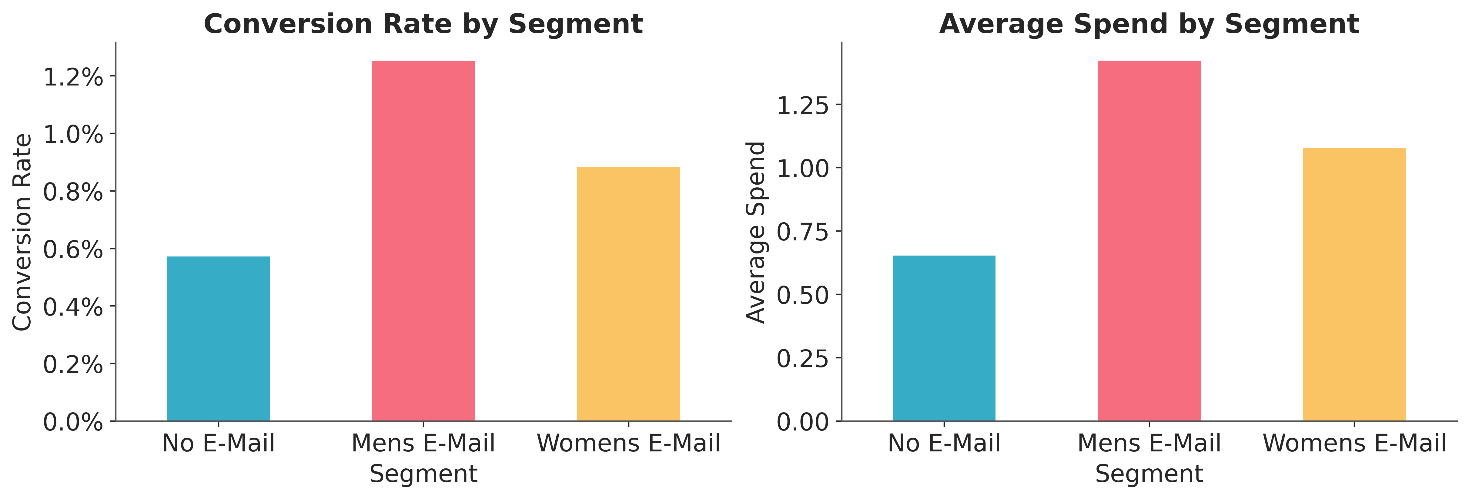
The email groups show higher conversion rates and spend than the control group.
fig, axes = plt.subplots(1, 2, figsize=(12, 4))

# All customers
for i, seg in enumerate(segments):
    subset = df.loc[df["segment"] == seg, "spend"]
    axes[0].hist(subset, label=seg, color=f"C{i}", density=True)
axes[0].set(xlabel="Spend", ylabel="Density")
axes[0].set_title("Spend Distribution (All Customers)")
axes[0].legend()

# Buyers only
for i, seg in enumerate(segments):
    subset = df.loc[(df["segment"] == seg) & (df["spend"] > 0), "spend"]
    axes[1].hist(subset, label=seg, color=f"C{i}", density=True)
axes[1].set(xlabel="Spend", ylabel="Density")
axes[1].set_title("Spend Distribution (Buyers Only)")
axes[1].legend();
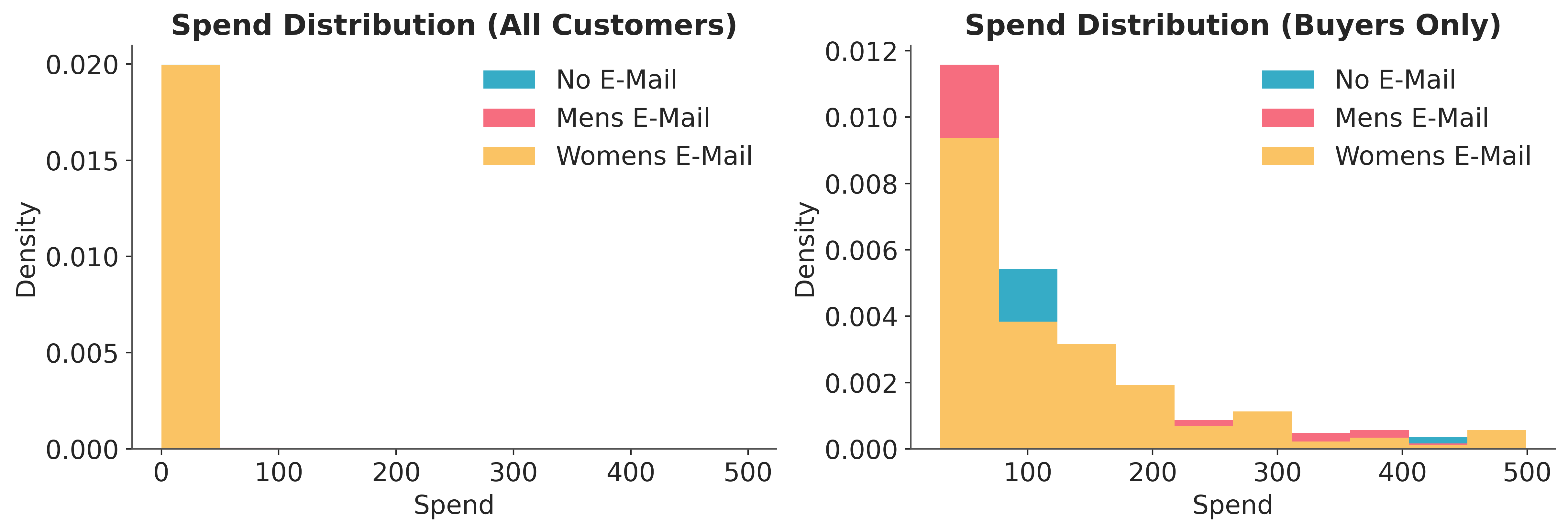
The left panel confirms that the spend distribution is heavily zero-inflated: the vast majority of customers do not purchase. The right panel, restricted to buyers, shows a right-skewed but roughly continuous distribution across all three segments.
Before modeling, we check that covariates are balanced across treatment arms, as expected in a randomized experiment.
balance_num = df.groupby("segment")[
    ["recency", "history", "mens", "womens", "newbie"]
].mean()

balance_cat = pd.concat(
    [
        pd.crosstab(df["segment"], df[col], normalize="index").rename(
            columns=lambda v, c=col: f"{c}: {v}",
        )
        for col in ["zip_code", "channel"]
    ],
    axis=1,
)

balance_num.join(balance_cat).round(2).T
| segment | Mens E-Mail | No E-Mail | Womens E-Mail |
|---|---|---|---|
| recency | 5.77 | 5.75 | 5.77 |
| history | 242.84 | 240.88 | 242.54 |
| mens | 0.55 | 0.55 | 0.55 |
| womens | 0.55 | 0.55 | 0.55 |
| newbie | 0.50 | 0.50 | 0.50 |
| zip_code: Rural | 0.15 | 0.15 | 0.15 |
| zip_code: Surburban | 0.45 | 0.45 | 0.45 |
| zip_code: Urban | 0.40 | 0.40 | 0.40 |
| channel: Multichannel | 0.12 | 0.12 | 0.12 |
| channel: Phone | 0.43 | 0.44 | 0.44 |
| channel: Web | 0.45 | 0.44 | 0.44 |
The means (for numeric covariates) and within-row proportions (for categorical covariates) are nearly identical across segments, confirming that the randomization worked as intended.
Note
Regarding causal identification, randomization ensures that treatment assignment is independent of potential outcomes, giving us ignorability (no confounding) and positivity by design. Consistency (a customer’s observed outcome equals the potential outcome under the assigned treatment) and no interference (one customer’s treatment does not affect another’s outcome) are not guaranteed by randomization and must be argued on domain grounds.
We encode the treatment segment as an integer, one-hot encode the categorical covariates, standardize the continuous ones for better sampling, and pack everything into JAX arrays.
# Map segment names to integer IDs for modeling
df["segment"] = df["segment"].map({name: i for i, name in enumerate(segments)})

# Dummy-encode categorical covariates
df = pd.get_dummies(
    df,
    columns=["zip_code", "channel"],
    drop_first=True,
    dtype=int,
)

# Standardize continuous covariates for better sampling
cols_to_standardize = ["recency", "history"]
df[cols_to_standardize] = (
    df[cols_to_standardize] - df[cols_to_standardize].mean()
) / df[cols_to_standardize].std(ddof=0)

# Build JAX arrays
segment = jnp.asarray(df["segment"].to_numpy(), dtype=jnp.int32)
X = jnp.asarray(
    df[
        ["recency", "history", "mens", "womens", "newbie"]
        + [c for c in df.columns if c.startswith(("zip_code_", "channel_"))]
    ].to_numpy(),
    dtype=jnp.float32,
)
y_conversion = jnp.asarray(df["conversion"].to_numpy(), dtype=jnp.int32)
y_spend = jnp.asarray(df["spend"].to_numpy(), dtype=jnp.float32)
Model 1: Conversion#
We model conversion as a Bayesian logistic regression. The linear predictor includes a global intercept, covariate effects, and a segment-specific shift that captures the treatment effect. The covariate coefficients are shared across treatment arms (no treatment x covariate interactions), so the treatment effect is homogeneous on the logit scale.
n_obs, n_features = X.shape


def conversion_model(X: Array, segment: Array, y: Array | None = None) -> None:
    alpha = sample("alpha", dist.Normal(0.0, 1.0))
    beta = sample("beta", dist.Normal(0.0, 1.0).expand([n_features]))
    tau = sample("tau", dist.Normal(0.0, 1.0).expand([len(segments)]))

    logit = alpha + X @ beta + tau[segment]

    with plate("obs", n_obs):
        sample("y", dist.Bernoulli(logits=logit), obs=y)
The parameter tau[0] corresponds to the control group (No E-Mail), tau[1]
to the Men’s E-Mail, and tau[2] to the Women’s E-Mail. The global intercept
alpha and segment shifts tau are not separately identifiable, but the
treatment-effect contrasts \(\tau_1 - \tau_0\) and \(\tau_2 - \tau_0\) are
always identified.
While those contrasts live on the logit scale, our target estimand is the Average
Treatment Effect (ATE) on the outcome scale, computed by predicting potential
outcomes under counterfactual treatment assignments and averaging over observations.
We wrap the model in an ImpactModel, which provides a unified interface
for fitting, prediction, and treatment-effect estimation.
Calling fit_on_batch() runs the configured inference engine
(here MCMC with the No-U-Turn Sampler) on the entire dataset in one pass.
rng_key, rng_subkey = random.split(rng_key)
im_conv = ImpactModel(
    conversion_model,
    rng_key=rng_subkey,
    inference=MCMC(
        NUTS(conversion_model),
        num_warmup=500,
        num_samples=500,
        num_chains=2,
    ),
)

im_conv.fit_on_batch(X, y_conversion, segment=segment)
After fitting, the underlying NumPyro inference object is accessible via
inference.
We use it here to print MCMC diagnostics.
azs.summary(az.from_numpyro(im_conv.inference))
| mean | sd | eti89_lb | eti89_ub | ess_bulk | ess_tail | r_hat | mcse_mean | mcse_sd | |
|---|---|---|---|---|---|---|---|---|---|
| alpha | -3.45 | 0.51 | -4.2 | -2.6 | 422 | 440 | 1.00 | 0.026 | 0.019 |
| beta[0] | -0.206 | 0.047 | -0.28 | -0.13 | 1091 | 563 | 1.00 | 0.0014 | 0.00097 |
| beta[1] | 0.187 | 0.039 | 0.12 | 0.25 | 756 | 677 | 1.00 | 0.0014 | 0.00096 |
| beta[2] | 0.29 | 0.122 | 0.1 | 0.49 | 585 | 405 | 1.00 | 0.0051 | 0.0036 |
| beta[3] | 0.42 | 0.118 | 0.23 | 0.62 | 527 | 480 | 1.00 | 0.0052 | 0.0037 |
| beta[4] | -0.436 | 0.088 | -0.57 | -0.3 | 920 | 661 | 1.00 | 0.0029 | 0.0021 |
| beta[5] | -0.32 | 0.11 | -0.5 | -0.14 | 813 | 668 | 1.00 | 0.0038 | 0.0026 |
| beta[6] | -0.245 | 0.109 | -0.43 | -0.074 | 740 | 719 | 1.00 | 0.004 | 0.0028 |
| beta[7] | -0.21 | 0.138 | -0.42 | 0.015 | 650 | 709 | 1.00 | 0.0054 | 0.0037 |
| beta[8] | -0.03 | 0.129 | -0.23 | 0.18 | 641 | 538 | 1.00 | 0.0052 | 0.0037 |
| tau[0] | -1.62 | 0.51 | -2.5 | -0.82 | 383 | 363 | 1.00 | 0.026 | 0.019 |
| tau[1] | -0.85 | 0.5 | -1.7 | -0.076 | 390 | 378 | 1.00 | 0.026 | 0.019 |
| tau[2] | -1.19 | 0.5 | -2 | -0.44 | 382 | 359 | 1.00 | 0.026 | 0.02 |
Before estimating treatment effects, we run a posterior predictive check to verify
that the model reproduces the observed conversion rates, overall and per treatment arm.
predict_on_batch() generates posterior predictive samples and
returns an DataTree.
dt_conv = im_conv.predict_on_batch(X, segment=segment)
dt_conv
<xarray.DataTree 'root'>
Group: /
├── Group: /posterior
│       Dimensions:     (chain: 1, draw: 1000, beta_dim_0: 9, tau_dim_0: 3)
│       Coordinates:
│         * chain       (chain) int64 8B 0
│         * draw        (draw) int64 8kB 0 1 2 3 4 5 6 7 ... 993 994 995 996 997 998 999
│         * beta_dim_0  (beta_dim_0) int64 72B 0 1 2 3 4 5 6 7 8
│         * tau_dim_0   (tau_dim_0) int64 24B 0 1 2
│       Data variables:
│           alpha       (chain, draw) float32 4kB -3.404 -3.697 -3.397 ... -2.4 -2.39
│           beta        (chain, draw, beta_dim_0) float32 36kB -0.1375 ... -0.2182
│           tau         (chain, draw, tau_dim_0) float32 12kB -1.71 -0.9072 ... -2.143
│       Attributes:
│           created_at:    2026-07-04T02:44:53.351583+00:00
│           aimz_version:  0.13.0
└── Group: /posterior_predictive
        Dimensions:  (chain: 1, draw: 1000, y_dim_0: 64000)
        Coordinates:
          * chain    (chain) int64 8B 0
          * draw     (draw) int64 8kB 0 1 2 3 4 5 6 7 ... 993 994 995 996 997 998 999
          * y_dim_0  (y_dim_0) int64 512kB 0 1 2 3 4 5 ... 63995 63996 63997 63998 63999
        Data variables:
            y        (chain, draw, y_dim_0) int32 256MB 0 0 0 0 0 0 0 ... 0 0 0 0 0 0 0
        Attributes:
            created_at:    2026-07-04T02:44:53.355890+00:00
aimz_version: 0.13.0pp_conv = dt_conv.posterior_predictive["y"]
fig, axes = plt.subplots(2, 2, figsize=(12, 8), layout="constrained")
axes = axes.flatten()
# Overall
obs_overall = float(y_conversion.mean())
pred_overall = pp_conv.mean(dim="y_dim_0").to_numpy().flatten()
axes[0].hist(pred_overall, bins=20, color="C0")
axes[0].axvline(
obs_overall,
color="red",
linestyle="--",
linewidth=2,
label=f"Obs: {obs_overall:.3f}",
)
axes[0].set_title("All")
axes[0].legend()
# Per treatment arm
for arm_id, arm_name in enumerate(segments):
mask = np.asarray(segment == arm_id)
obs_arm = float(y_conversion[mask].mean())
pred_arm = pp_conv.isel(y_dim_0=mask).mean(dim="y_dim_0").to_numpy().flatten()
axes[arm_id + 1].hist(pred_arm, bins=20, color=f"C{arm_id + 1}")
axes[arm_id + 1].axvline(
obs_arm,
color="red",
linestyle="--",
linewidth=2,
label=f"Obs: {obs_arm:.3f}",
)
axes[arm_id + 1].set_title(arm_name)
axes[arm_id + 1].legend()
fig.supxlabel("Mean Predicted Rate")
fig.supylabel("Frequency")
fig.suptitle(
"Posterior Predictive Check: Conversion",
fontsize=18,
fontweight="bold",
y=1.05,
);
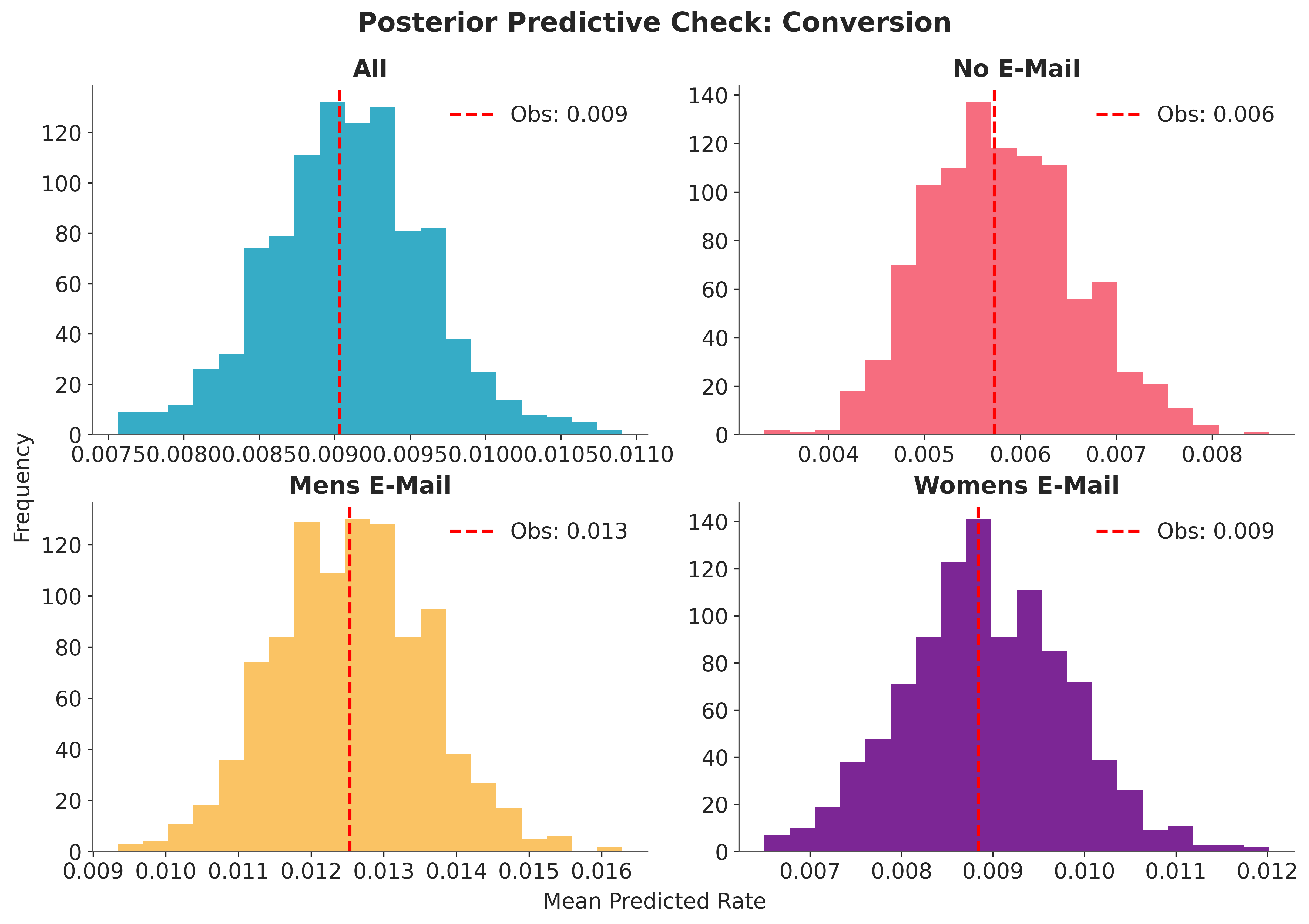
The observed rate (red dashed line) falls within the bulk of the posterior predictive distribution for each arm, indicating an adequate fit.
Estimating Treatment Effects on Conversion#
With the fitted model in hand, we now estimate treatment effects.
estimate_effect() takes two scenarios, each a dict of keyword
arguments that would be passed to the underlying prediction method.
For every posterior draw, it generates predictions under both scenarios, subtracts
baseline from intervention, and returns per-observation differences as an
DataTree.
Because segment is a function argument rather than a
sample() site, each counterfactual scenario is
specified by passing the desired treatment value directly.
effect_conv_mens = im_conv.estimate_effect(
    args_baseline={
        "X": X,
        "segment": jnp.zeros(n_obs, dtype=jnp.int32),
    },
    args_intervention={
        "X": X,
        "segment": jnp.ones(n_obs, dtype=jnp.int32),
    },
    on_batch=True,
)

effect_conv_womens = im_conv.estimate_effect(
    args_baseline={
        "X": X,
        "segment": jnp.zeros(n_obs, dtype=jnp.int32),
    },
    args_intervention={
        "X": X,
        "segment": 2 * jnp.ones(n_obs, dtype=jnp.int32),
    },
    on_batch=True,
)
Averaging the per-observation differences over all customers gives the ATE posterior, one value per draw, fully propagating parameter uncertainty.
ate_conv_mens = effect_conv_mens.posterior_predictive["y"].mean(dim="y_dim_0")
ate_conv_womens = effect_conv_womens.posterior_predictive["y"].mean(dim="y_dim_0")
We plot the ATE posteriors for both campaigns alongside the posterior mean and a zero-effect reference.
fig, axes = plt.subplots(1, 2, figsize=(12, 4), layout="constrained")

for i, (ax, ate, label) in enumerate(
    zip(
        axes,
        [ate_conv_mens, ate_conv_womens],
        ["Mens E-Mail vs. No E-Mail", "Womens E-Mail vs. No E-Mail"],
        strict=True,
    ),
):
    pp_ate = ate.to_numpy().flatten()
    ax.hist(pp_ate, bins=20, color=f"C{i}")
    mean = pp_ate.mean()
    ax.axvline(
        mean,
        color="red",
        linestyle="--",
        linewidth=2,
        label=f"Mean: {mean:.3f}",
    )
    ax.axvline(0, color="gray", linestyle=":")
    ax.set_title(label)
    ax.legend()

fig.supxlabel("ATE (Conversion Rate)")
fig.supylabel("Frequency")
fig.suptitle(
    "Treatment Effects: Conversion",
    fontsize=18,
    fontweight="bold",
    y=1.1,
);
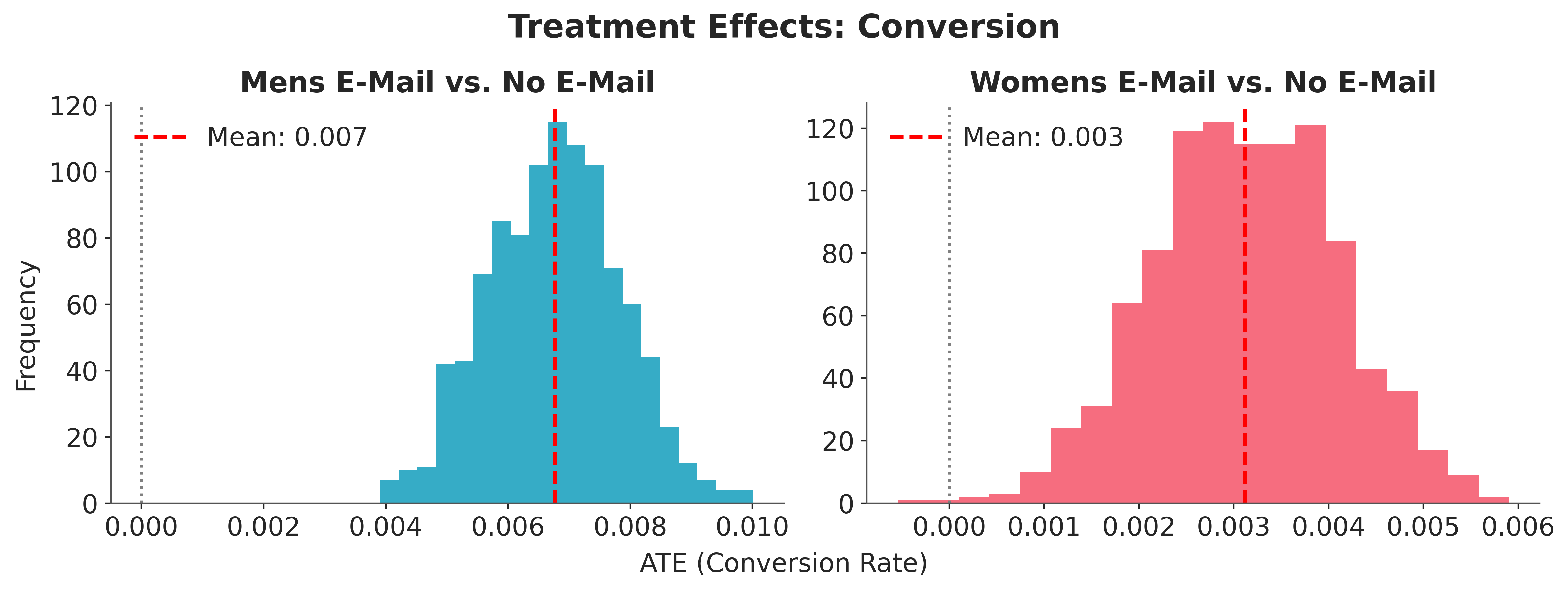
Both posterior distributions sit entirely above zero, providing strong evidence that both campaigns increase conversion relative to the control group. The Men’s E-Mail effect is somewhat larger, though the posteriors overlap substantially.
Model 2: Spend#
Spend is zero for most customers and right-skewed among buyers. We use a hurdle model with two components: a Bernoulli gate for whether the customer purchases at all, and a log-normal distribution for the spend amount conditional on purchasing.
This model demonstrates how ImpactModel handles custom likelihoods.
Because the hurdle likelihood does not decompose into a single
sample() statement, we compute the log-likelihood manually and
register it with factor() during fitting.
At prediction time, we switch to the generative form: sample purchase from
the Bernoulli, sample amount from the log-normal distribution, and return their
product as y.
def spend_model(X: Array, segment: Array, y: Array | None = None) -> None:
    # --- Hurdle component: P(spend > 0) ---
    alpha_h = sample("alpha_h", dist.Normal(-5.0, 1.0))
    beta_h = sample("beta_h", dist.Normal(0.0, 1.0).expand([n_features]))
    tau_h = sample("tau_h", dist.Normal(0.0, 1.0).expand([len(segments)]))
    logit = alpha_h + X @ beta_h + tau_h[segment]

    # --- Amount component: log(spend) | spend > 0 ---
    alpha_a = sample("alpha_a", dist.Normal(5.0, 1.0))
    beta_a = sample("beta_a", dist.Normal(0.0, 1.0).expand([n_features]))
    tau_a = sample("tau_a", dist.Normal(0.0, 1.0).expand([len(segments)]))
    sigma = sample("sigma", dist.HalfNormal(1.0))
    mu = alpha_a + X @ beta_a + tau_a[segment]

    if y is not None:
        is_zero = y == 0.0
        with plate("obs", n_obs):
            log_lik = jnp.where(
                is_zero,
                jax.nn.log_sigmoid(-logit),
                jax.nn.log_sigmoid(logit)
                + dist.LogNormal(mu, sigma).log_prob(jnp.where(is_zero, 1.0, y)),
            )
            factor("y", log_lik)
    else:
        with plate("obs", n_obs):
            purchase = sample("purchase", dist.Bernoulli(logits=logit))
            amount = sample("amount", dist.LogNormal(mu, sigma))
            deterministic("y", purchase * amount)
The intercepts are centered on domain-appropriate values for each component: a low baseline purchase probability for the hurdle, and a plausible log-scale spend level for the amount.
We fit the hurdle model using the same MCMC configuration as before.
rng_key, rng_subkey = random.split(rng_key)
im_spend = ImpactModel(
    spend_model,
    rng_key=rng_subkey,
    inference=MCMC(
        NUTS(spend_model),
        num_warmup=500,
        num_samples=500,
        num_chains=2,
    ),
)

im_spend.fit_on_batch(X, y_spend, segment=segment)
MCMC diagnostics:
azs.summary(az.from_numpyro(im_spend.inference))
| mean | sd | eti89_lb | eti89_ub | ess_bulk | ess_tail | r_hat | mcse_mean | mcse_sd | |
|---|---|---|---|---|---|---|---|---|---|
| alpha_a | 4.57 | 0.52 | 3.7 | 5.4 | 461 | 571 | 1.01 | 0.024 | 0.017 |
| alpha_h | -4.87 | 0.54 | -5.7 | -4 | 454 | 511 | 1.00 | 0.025 | 0.018 |
| beta_a[0] | 0.031 | 0.037 | -0.028 | 0.09 | 1141 | 646 | 1.00 | 0.0011 | 0.00074 |
| beta_a[1] | 0.009 | 0.035 | -0.047 | 0.066 | 1157 | 615 | 1.01 | 0.001 | 0.00073 |
| beta_a[2] | 0.037 | 0.103 | -0.13 | 0.2 | 873 | 837 | 1.00 | 0.0035 | 0.0023 |
| beta_a[3] | -0.176 | 0.104 | -0.34 | -0.011 | 911 | 847 | 1.00 | 0.0035 | 0.0023 |
| beta_a[4] | 0.04 | 0.074 | -0.076 | 0.16 | 1308 | 753 | 1.00 | 0.0021 | 0.0017 |
| beta_a[5] | 0.046 | 0.097 | -0.11 | 0.2 | 1064 | 855 | 1.01 | 0.003 | 0.002 |
| beta_a[6] | 0.05 | 0.098 | -0.099 | 0.21 | 933 | 674 | 1.00 | 0.0032 | 0.0023 |
| beta_a[7] | 0.076 | 0.109 | -0.1 | 0.24 | 1059 | 569 | 1.00 | 0.0033 | 0.0025 |
| beta_a[8] | 0.028 | 0.105 | -0.14 | 0.19 | 1113 | 786 | 1.01 | 0.0031 | 0.0023 |
| beta_h[0] | -0.208 | 0.045 | -0.28 | -0.14 | 1382 | 720 | 1.00 | 0.0012 | 0.00087 |
| beta_h[1] | 0.184 | 0.04 | 0.12 | 0.25 | 747 | 628 | 1.01 | 0.0015 | 0.0011 |
| beta_h[2] | 0.351 | 0.122 | 0.16 | 0.55 | 879 | 859 | 1.00 | 0.0041 | 0.0029 |
| beta_h[3] | 0.482 | 0.125 | 0.29 | 0.69 | 859 | 653 | 1.00 | 0.0043 | 0.003 |
| beta_h[4] | -0.424 | 0.091 | -0.57 | -0.28 | 1333 | 847 | 1.00 | 0.0025 | 0.0018 |
| beta_h[5] | -0.289 | 0.118 | -0.48 | -0.11 | 959 | 951 | 1.00 | 0.0038 | 0.0025 |
| beta_h[6] | -0.211 | 0.119 | -0.39 | -0.019 | 1090 | 712 | 1.00 | 0.0036 | 0.0024 |
| beta_h[7] | -0.173 | 0.13 | -0.39 | 0.04 | 1015 | 728 | 1.00 | 0.0041 | 0.0029 |
| beta_h[8] | 0.008 | 0.122 | -0.18 | 0.2 | 978 | 720 | 1.00 | 0.0039 | 0.003 |
| sigma | 0.839 | 0.0243 | 0.8 | 0.88 | 1609 | 663 | 1.01 | 0.00061 | 0.00043 |
| tau_a[0] | -0.17 | 0.51 | -0.95 | 0.67 | 461 | 573 | 1.00 | 0.024 | 0.017 |
| tau_a[1] | -0.24 | 0.51 | -1.1 | 0.62 | 451 | 528 | 1.00 | 0.024 | 0.017 |
| tau_a[2] | -0.1 | 0.51 | -0.91 | 0.75 | 449 | 532 | 1.00 | 0.024 | 0.017 |
| tau_h[0] | -0.34 | 0.53 | -1.2 | 0.49 | 448 | 501 | 1.00 | 0.025 | 0.017 |
| tau_h[1] | 0.44 | 0.53 | -0.44 | 1.3 | 440 | 436 | 1.00 | 0.025 | 0.018 |
| tau_h[2] | 0.09 | 0.53 | -0.77 | 0.94 | 445 | 479 | 1.00 | 0.025 | 0.017 |
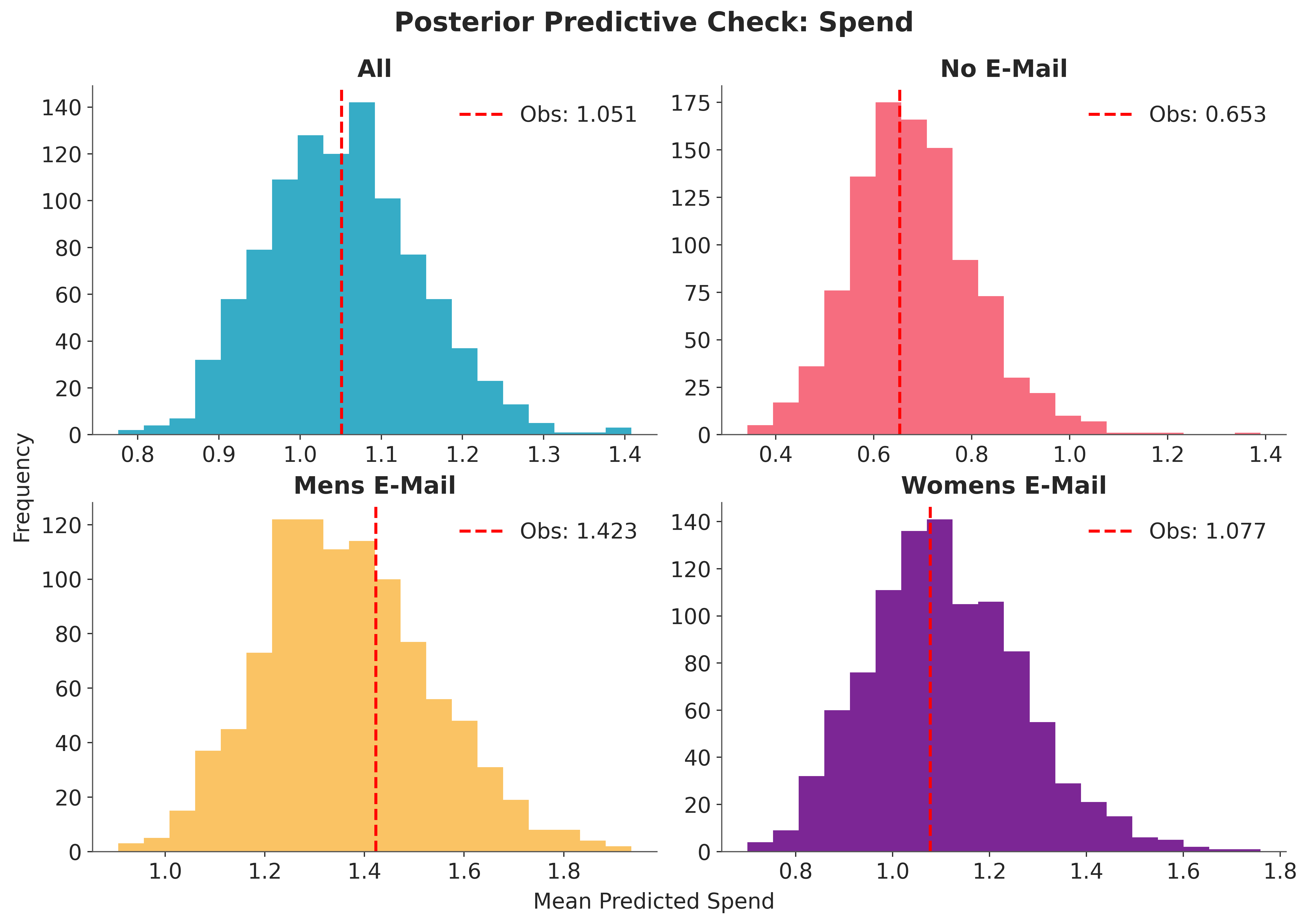
Following the same workflow as the conversion model, we check that the predicted spend matches the observed values per arm.
dt_spend = im_spend.predict_on_batch(X, segment=segment)
pp_spend = dt_spend.posterior_predictive["y"]

fig, axes = plt.subplots(2, 2, figsize=(12, 8), layout="constrained")
axes = axes.flatten()

# Overall
obs_overall = float(y_spend.mean())
pred_overall = pp_spend.mean(dim="y_dim_0").to_numpy().flatten()
axes[0].hist(pred_overall, bins=20, color="C0")
axes[0].axvline(
    obs_overall,
    color="red",
    linestyle="--",
    linewidth=2,
    label=f"Obs: {obs_overall:.3f}",
)
axes[0].set_title("All")
axes[0].legend()

# Per treatment arm
for arm_id, arm_name in enumerate(segments):
    mask = np.asarray(segment == arm_id)
    obs_arm = float(y_spend[mask].mean())
    pred_arm = pp_spend.isel(y_dim_0=mask).mean(dim="y_dim_0").to_numpy().flatten()
    axes[arm_id + 1].hist(pred_arm, bins=20, color=f"C{arm_id + 1}")
    axes[arm_id + 1].axvline(
        obs_arm,
        color="red",
        linestyle="--",
        linewidth=2,
        label=f"Obs: {obs_arm:.3f}",
    )
    axes[arm_id + 1].set_title(arm_name)
    axes[arm_id + 1].legend()

fig.supxlabel("Mean Predicted Spend")
fig.supylabel("Frequency")
fig.suptitle(
    "Posterior Predictive Check: Spend",
    fontsize=18,
    fontweight="bold",
    y=1.05,
);
Estimating Treatment Effects on Spend#
We repeat the same counterfactual procedure as for conversion, now using the spend model.
effect_spend_mens = im_spend.estimate_effect(
    args_baseline={
        "X": X,
        "segment": jnp.zeros(n_obs, dtype=jnp.int32),
    },
    args_intervention={
        "X": X,
        "segment": jnp.ones(n_obs, dtype=jnp.int32),
    },
    on_batch=True,
)

effect_spend_womens = im_spend.estimate_effect(
    args_baseline={
        "X": X,
        "segment": jnp.zeros(n_obs, dtype=jnp.int32),
    },
    args_intervention={
        "X": X,
        "segment": 2 * jnp.ones(n_obs, dtype=jnp.int32),
    },
    on_batch=True,
)
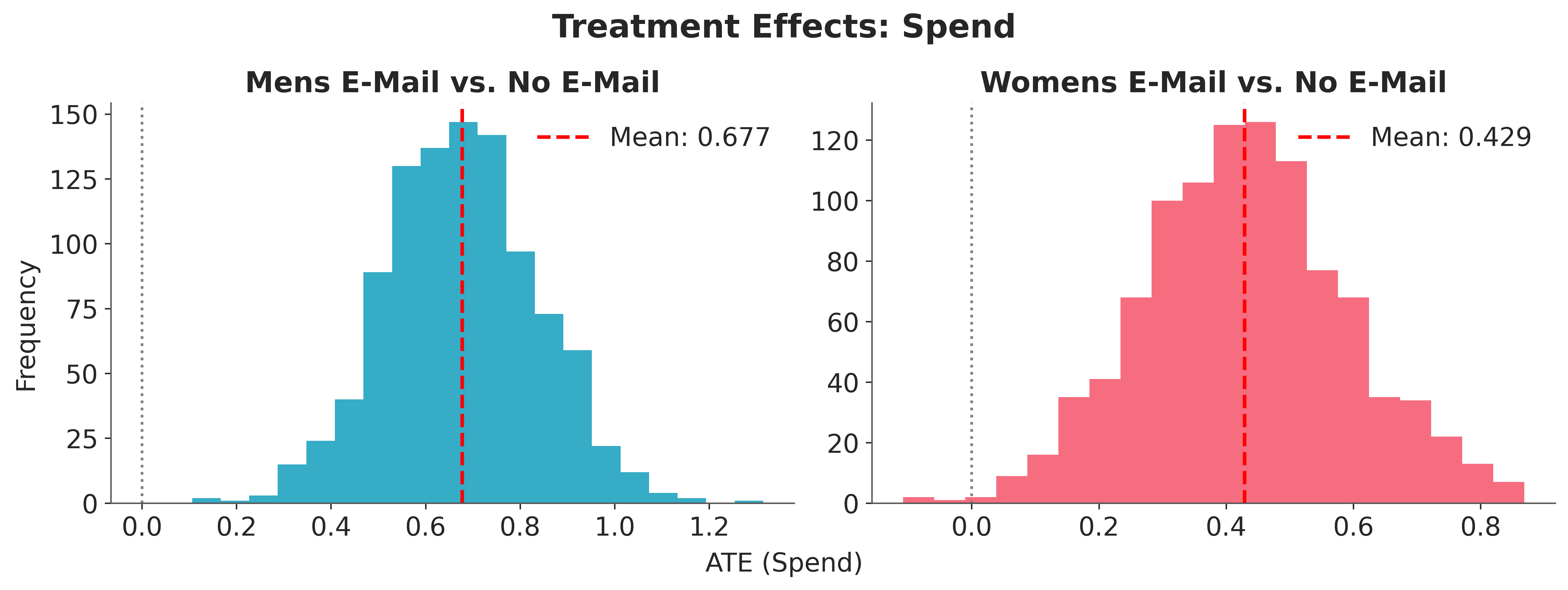
Averaging per-observation spend differences gives the ATE posterior in dollars.
ate_spend_mens = effect_spend_mens.posterior_predictive["y"].mean(dim="y_dim_0")
ate_spend_womens = effect_spend_womens.posterior_predictive["y"].mean(dim="y_dim_0")
We visualize the spend ATE posteriors for both campaigns.
fig, axes = plt.subplots(1, 2, figsize=(12, 4), layout="constrained")

for i, (ax, ate, label) in enumerate(
    zip(
        axes,
        [ate_spend_mens, ate_spend_womens],
        ["Mens E-Mail vs. No E-Mail", "Womens E-Mail vs. No E-Mail"],
        strict=True,
    ),
):
    pp_ate = ate.to_numpy().flatten()
    ax.hist(pp_ate, bins=20, color=f"C{i}")
    mean = pp_ate.mean()
    ax.axvline(
        mean,
        color="red",
        linestyle="--",
        linewidth=2,
        label=f"Mean: {mean:.3f}",
    )
    ax.axvline(0, color="gray", linestyle=":")
    ax.set_title(label)
    ax.legend()

fig.supxlabel("ATE (Spend)")
fig.supylabel("Frequency")
fig.suptitle(
    "Treatment Effects: Spend",
    fontsize=18,
    fontweight="bold",
    y=1.1,
);
Comparison#
We compare treatment effects across both outcomes to check whether the campaigns that drive more conversions also drive more revenue.
fig, axes = plt.subplots(1, 2, figsize=(12, 4), sharey=True)

# Conversion effects
for i, ate in enumerate([ate_conv_mens, ate_conv_womens]):
    pp_ate = ate.to_numpy().flatten()
    mean = pp_ate.mean()
    hdi = azs.hdi(pp_ate)
    axes[0].errorbar(
        mean, i,
        xerr=[[mean - hdi[0]], [hdi[1] - mean]],
        fmt="o", capsize=5, color="C0", markersize=8,
    )
axes[0].set_yticks(range(2))
axes[0].set_yticklabels(["Men's vs. No E-Mail", "Women's vs. No E-Mail"])
axes[0].axvline(0, color="gray", linestyle=":")
axes[0].set_xlabel("ATE (Conversion Rate)")
axes[0].set_title("Conversion")

# Spend effects
for i, ate in enumerate([ate_spend_mens, ate_spend_womens]):
    pp_ate = ate.to_numpy().flatten()
    mean = pp_ate.mean()
    hdi = azs.hdi(pp_ate)
    axes[1].errorbar(
        mean, i,
        xerr=[[mean - hdi[0]], [hdi[1] - mean]],
        fmt="o", capsize=5, color="C1", markersize=8,
    )
axes[1].axvline(0, color="gray", linestyle=":")
axes[1].set_xlabel("ATE (Spend)")
axes[1].set_title("Spend")

fig.suptitle("Treatment Effect Comparison", fontsize=18, fontweight="bold");
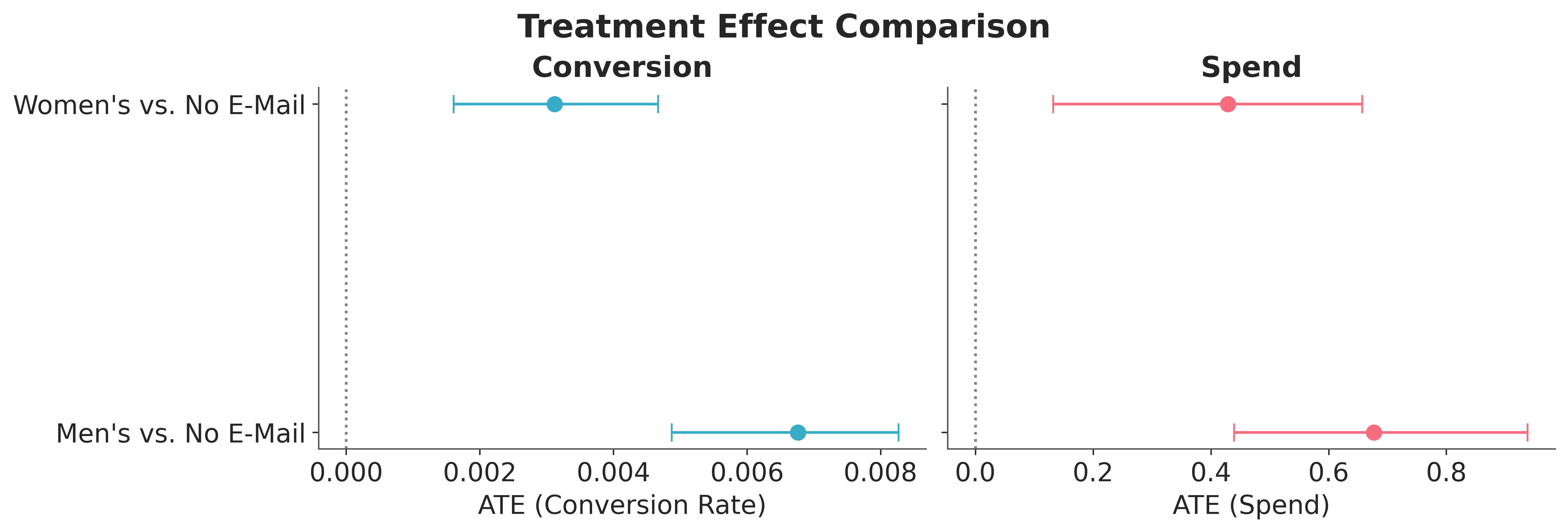
Both campaigns increase conversion and spend relative to the control, and the Men’s campaign shows a larger effect on both outcomes.
References#
Freedman, D. A. (2008). On regression adjustments to experimental data. Advances in Applied Mathematics, 40(2), 180–193.
Hillstrom, K. (2008). The MineThatData E-Mail Analytics and Data Mining Challenge. MineThatData Blog.